Extreme Physics at Extreme Baselines Andrei Lobanov, MPIfR Bonn - - PowerPoint PPT Presentation

Extreme Physics at Extreme Baselines

Andrei Lobanov, MPIfR Bonn

2

VLBI View of AGN Jets

 SVLBI and mmVLBI are best direct probes of physics of central engine in AGN: Tb, polarization, magnetic field.

5 RS

Poynting flux dominated Launching region Kinetic flux dominated 50 µas in M87

RA, 22GHz VLBI, 215GHz VLBA, 43GHz VLBI, 86GHz

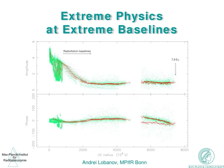
 RadioAstron has extended interferometric baselines to uv- spacings of up to 15 Gλ. EHT reaches up to ~8 Gλ. Both venture into truly uncharted domains.  Narrow range of PA covered by RA space baselines: may be problematic for analysis and even detection.

Uncharted Territory ...

Gómez et al. 2015; talk by Jose Luis tomorrow

 The jets are strongly resolved in RA images. What you see are the brighter „threads“ inside the flow. What are their properties? Polarization, spectrum, and Tb should tell this.

... and its Maps

Vega Garcia et al. 2016; talks by Laura, Manel, and Tuomas

 „A temperature is a comparative objective measure of ... hot and cold“ (Wikipedia).  ... a microscopic measure of kinetic (thermal) energy stored.  Brightness temperature is a black body temperature needed to emulate what you see from you favorite (not so black) body – e.g., in the Planck regime:

• r in the Rayleigh-Taylor regime

(Brightness) Temperature

 You want to have Iν, but really measure S over an area Ω.  If you don‘t care about the extent of your region, you need to care about the resolution limit of your instrument. Then  Otherwise, you need to image or model the structure of interest, before you can estimate Tb. Take, for instance (as everybody does) an elliptical gaussian:

Getting to that Iν

1) Tough luck, except if you are doing interferometry. 2) Reality of life, if you are doing tough interferometry.  Tough interferometry:

• - space, mm-, submm- VLBI
• - optical interferometry (often)
• - snapshot observations (e.g., geodetic VLBI)

 Interferometrist‘s luck: V(q) = F I(r) Measure S (proxied by V) and θ (proxied by q-1) with every single visibility.  Use it or lose it!

What If I Can‘t Make That Image?

 ... must be very easy: 𝑈𝑐 =

𝐽𝜉𝑑2 2𝑙 𝜉2 = 𝑇 𝜇2 2𝑙 Ω .

• - Make a single measurement of V on a baseline B.
• - Take the proxies 𝑇 → 𝑊 and 𝜄 → 1/𝑟 (Ω → 𝜌

𝑟2

)

• - Recall that 𝑟 = 𝐶

𝜇

⁄ And you’ll get 𝑈𝑐 =

𝐽𝜉𝑑2 2𝑙 𝜉2 = 𝑊 𝐶2 2𝜌 𝑙

Feeling Lucky

We’re done! Let’s go and have some party!

 ... comes in different shapes, and is also noisy (σq)  Hence you need to know something about V(q) at least at two different values of q. For instance, V0 = V(q)|q=0.  Then you can use 𝑊

𝑟 < 𝑊 0 and 𝑊 𝑟 + 𝜏𝑟 ≤ 𝑊 0 to constrain 𝑈𝑐.

That Darn V (q)= V q exp(-i φq)

 by taking V0 for a ride... and dropping it underway.  All you need for this is to assume a shape, for instance, a Gaussian, or a disk, or a shell – whatever comes close to the physical reality of your target.  For example, for a Gaussian, one has: and you see now why 𝑈𝑐 =

𝑊

𝑟 𝐶2

2𝜌 𝑙 was a bad idea.

...Well, let‘s also see if we can get rid of V0

Let‘s Commit a Treason

 while picking one‘s favorite value of V0?  Indeed, there is always a minimum of Tb, realized for some V0>Vq, since 𝑈𝑐 → ∞ for 𝑊

0 → 𝑊 𝑟 and 𝑊 0 → ∞.

 It‘s at 𝑊

0 = 𝑓 𝑊 𝑟

for the Gaussian.  So, for a given Vq, you cannot get brightness temper- ature smaller than no matter how hard you may try. (And we‘re halfway there.)

How Low Can One Fall...

How High Can One Climb...

 while going away from 𝑊

0 = 𝑓 𝑊 𝑟?

 Possible answers: 𝑊

0 → ∞ (yahoo!)

𝑊

0 = 𝑇tot (not good)

𝑊

0 = 𝑊 𝑟 + 𝜏𝑟 (perhaps,

the better one)  Then, you‘d get:

 A single visibility amplitude, Vq, and its error, σq, measured at a spatial frequency, q, are sufficient for obtaining estimates of the minimum brightness temperature, and an upper limit of a brightness temperature under the assumption that the structure is resolved at the spatial frequency of the measurement.  Specific expressions for other patterns of brightness distributions can also be derived (see A&A, 574, 84).

A One-Slide Recap

Brightness Temperature Runs

 ... well within the (Tb,min,Tb,lim) bracket, at all q > 200Mλ

 ... for a jet dominated object (NGC 1052)

And It Does That Even Better

 Test on MOJAVE data (Tb from elliptical Gaussian model fits of the compact cores; Kovalev+2005)  Compare with Tb,lim from 1% of the longest baselines

Prove It For The Masses!

 What if Tb is determined by transverse size of the jet?

Doctoring the Proof

 Yes, we can! Too low Tb estimates may result from (unjustifiably) taking too much of the extended structure on board.

Can We Fail w ith Model Fit?

 ... only makes things better. Just look at direct comparison with 3mm VLBI data (Lee+2008), made at B > 2 Gλ

Trying It at Gigalambdas

 Most of the AGN imaged with RA show 𝑈𝑐,𝑛𝑛𝑛 ≥ 1013 K and 𝑈𝑐,𝑚𝑛𝑛 ≥ 1014 K  Both are well above the IC limit on brightness temperature.

What Do We Get from RadioAstron?

Lobanov et al. 2015 Gómez et al. 2015

0642+449 BL Lac

 Seemingly, calibration errors should have yielded too low Tb as well, but they didn‘t – more systematic analysis is in Yuri‘s talk on the RadioAstron AGN survey.  Let‘s see what can we do to get those high Tb values:  Eery... the right column could very well describe... a pulsar!

• r, generically, a highly magnetized object. If so, we may

expect high Tb to be accompanied by high magnetic field.

New Physics or Old Calibration Errors?

Tb ~ 1012 K Tb >> 1012 K Emitting particles: e- e+ e- p+ Emission: incoherent coherent Particle distribution: power law

• > monoenergetic

Physical conditions: ~ equilibrium continued injection Geometrical conditions:

• utside of jet cone

inside of jet cone

 Taking a look at a „normal“ IC-loss dominated plasma in a strong magnetic field gives: 𝑈𝑐,𝑛𝑛𝑛 ~ 7 × 109 K 𝐶3/4 G  This, of course, implies a sky-rocketing 𝜉𝑛 ∝ 𝐶1/2.  However, the rogue 𝜉𝑛 can be kept low if the plasma particle density 𝑂0 ∝ 𝐶−7/2.  This is actualy pretty feasible for: – a „runaway“ TEMZ cell; – a BZ beam inside of BP jet; – a truly „indigenous“ pair creation (for 𝐶 > 1013 G)

What if You Crank Up the B?

 A measurement of visibility amplitude, Vq, alone is sufficient to derive an estimate of the minimum brightness temperature, Tb,min.  A measurement of Vq and its error σq provides an estimate

• f limiting brightness temperature, Tb,lim, under the

requirement of the structure to be marginally resolved at the spatial frequency of measurement.  The range (Tb,min, Tb,lim) provides a good bracket for Tb when measurements are done at q>200 Mλ.  In some cases (elongated or overly resolved structures), Tb,lim is a better estimate of the maximum brightness temperature.

Bottom Lines

 The RA estimates of Tb,min imply B > 105 G.  Good evidence for B~ 103—104 G in the nuclear region (recall presentation by Anne-Kathrin).  Perhaps even stronger fields are implied by RM > 108 rad/m2 measured with ALMA (Marti-Vidal+ 2015).  Even higher magnetic fields can be expected for exotic

• bjects such as magnetized rotators (Kardashev 1995) or

gravastars (Mazur & Mottola 2001).  The quest for high Tb must therefore continue!

Bs and T bs in AGN