
SLIDE 1
1
Class #06: Evaluating ML Algorithms
Machine Learning (COMP 135): M. Allen, 23 Sept. 19
Binary and Other Classification
} We will generally discuss binary classifiers, which divide
data into one of two classes
} Recall: we label these classes 1 and 0 for convenience
} Many of the things we discuss can be applied to more
than two classes, however
} Decision trees “don’t care” how many class labels there are,
and nothing in the information-theoretic heuristic, or many
- thers, depends upon this
} Linear classifiers as presented in last lecture are inherently
binary, defining the classes based on two regions, determined relative to a linear function
Monday, 23 Sep. 2019 Machine Learning (COMP 135) 2
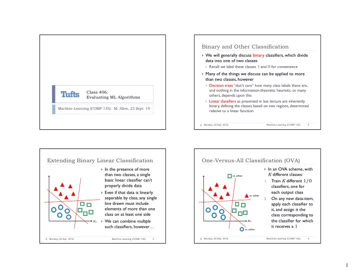
Extending Binary Linear Classification
} In the presence of more
than two classes, a single basic linear classifier can’t properly divide data
} Even if that data is linearly
separable by class, any single line drawn must include elements of more than one class on at least one side
} We can combine multiple
such classifiers, however…
Monday, 23 Sep. 2019 Machine Learning (COMP 135) 3
x1
One-Versus-All Classification (OVA)
} In an OVA scheme, with
K different classes:
1.
Train K different 1/0 classifiers, one for each output class
2.
On any new data-item, apply each classifier to it, and assign it the class corresponding to the classifier for which it receives a 1
Monday, 23 Sep. 2019 Machine Learning (COMP 135) 4
x1
- vs. other
- vs. other
- vs. other