SLIDE 1 Exercise C2-41
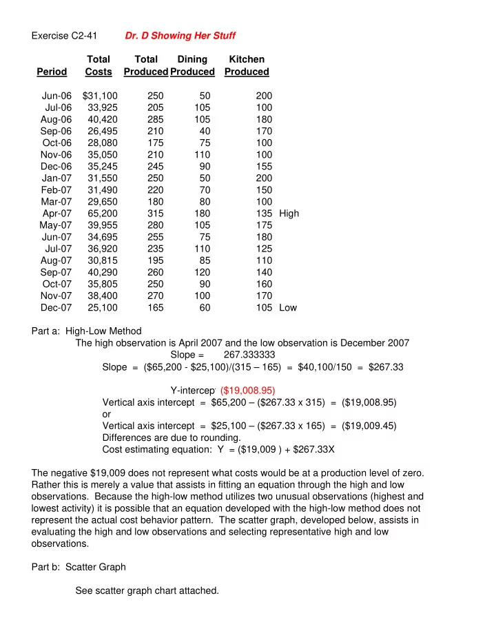
Total Total Dining Kitchen Period Costs Produced Produced Produced Jun-06 $31,100 250 50 200 Jul-06 33,925 205 105 100 Aug-06 40,420 285 105 180 Sep-06 26,495 210 40 170 Oct-06 28,080 175 75 100 Nov-06 35,050 210 110 100 Dec-06 35,245 245 90 155 Jan-07 31,550 250 50 200 Feb-07 31,490 220 70 150 Mar-07 29,650 180 80 100 Apr-07 65,200 315 180 135 High May-07 39,955 280 105 175 Jun-07 34,695 255 75 180 Jul-07 36,920 235 110 125 Aug-07 30,815 195 85 110 Sep-07 40,290 260 120 140 Oct-07 35,805 250 90 160 Nov-07 38,400 270 100 170 Dec-07 25,100 165 60 105 Low Part a: High-Low Method The high observation is April 2007 and the low observation is December 2007 Slope = 267.333333 Slope = ($65,200 - $25,100)/(315 – 165) = $40,100/150 = $267.33 Y-intercept ($19,008.95) Vertical axis intercept = $65,200 – ($267.33 x 315) = ($19,008.95)
Vertical axis intercept = $25,100 – ($267.33 x 165) = ($19,009.45) Differences are due to rounding. Cost estimating equation: Y = ($19,009 ) + $267.33X The negative $19,009 does not represent what costs would be at a production level of zero. Rather this is merely a value that assists in fitting an equation through the high and low
- bservations. Because the high-low method utilizes two unusual observations (highest and
lowest activity) it is possible that an equation developed with the high-low method does not represent the actual cost behavior pattern. The scatter graph, developed below, assists in evaluating the high and low observations and selecting representative high and low
Part b: Scatter Graph See scatter graph chart attached.
SLIDE 2 S r n S S
It appears the April 2007 observation is not representative of normal operating conditions and should be excluded from an analysis of costs under normal operating conditions. Part c: Excluding April 2007 from results The high observation is August 2006 and the low observation is December 2007 Slope = $127.67 Slope = ($40,420 - $25,100)/(285 – 165) = $15,320/120 = $127.67 Y-intercept $4,034.05 Vertical axis intercept = $40,420 – ($127.67 x 285) = $4,034.05
Vertical axis intercept = $25,100 – ($127.67 x 165) = $4,034.45 Differences are due to rounding. Cost estimating equation: Y = $4,034 + $127.67X The results are strikingly different from those obtained in part “a.” The vertical axis intercept is much higher, and a positive number, while the slope is smaller. Basically, the unusual high observation in part “a” pulled the high end of the equation up from what is should be. How do these new results compare with the scatter graph? Let's recompute the scatter graph excluding April 2007. Part d: Regression Analysis (omitting April 2007)
SUMMARY OUTPUT Regression Statistics Multiple R 0.82664428 R Square 0.68334076 Adjusted R 0.66354956 Standard E 2699.30168 Observatio 18 ANOVA df SS MS F ignificance F Regression 1 251575301 251575301 34.52750146 2.344E-05 Residual 16 116579673 7286229.5 Total 17 368154974 Coefficients tandard Err t Stat P-value Intercept 9343.75123 4178.4837 2.2361584 0.039937683 X Variable 105.506637 17.955488 5.8760107 2.34376E-05
The cost estimating equation is: Y = $9,343.751 + 105.51X
SLIDE 3 S r n S S
2
This equation has two advantages over that developed in part “c.” It uses all observations (except April 2007), rather than just two representative
- bservations. It provides information on how well the cost estimating equation
explains the variation in the dependent variable. In this case, the cost estimating equation explains 68.3341 percent of the variation in total manufacturing costs. Because of the least-squares criteria, the analyst must evaluate the data used in regression analysis and exclude unusual observations. Otherwise, a single large squared deviation will have a disproportionate influence in the cost estimating equation. Part e: If we assume that the slope is the marginal cost of producing a table, should we accept the offer of $180 per table? In all cases, $180 > slope … so why not? So far we've assumed that all tables (both dining and kitchen) cost the same to produce. What if that's not true? We may make a bad decision if we accept $180 for a dining room table. We can repeat our regression analysis using both dining and kitchen tables as separate X variables.
SUMMARY OUTPUT Regression Statistics Multiple R 0.99854387 R Square 0.99708986 Adjusted R 0.99670185 Standard E 267.255328 Observatio 18 ANOVA df SS MS F ignificance F Regression 2 367083592 183541796 2569.698867 9.536E-20 Residual 15 1071381.2 71425.41 Total 17 368154974 Coefficients tandard Err t Stat P-value Intercept 5269.61864 425.93186 12.371976 2.84498E-09 X Variable 197.242549 2.8920908 68.200675 4.07986E-20 X Variable 80.2760267 1.8852195 42.581793 4.61031E-17
Now it appears that our marginal cost for a dining room table is $197.24. If we agreed to a price of $180 per table, we'd lose $17.24 per table sold. Management should reject the offer.
SLIDE 4
Data Excluding April 2007 Jun-06 $31,100 250 50 200 Jul-06 33,925 205 105 100 Aug-06 40,420 285 105 180 Sep-06 26,495 210 40 170 Oct-06 28,080 175 75 100 Nov-06 35,050 210 110 100 Dec-06 35,245 245 90 155 Jan-07 31,550 250 50 200 Feb-07 31,490 220 70 150 Mar-07 29,650 180 80 100 May-07 39,955 280 105 175 Jun-07 34,695 255 75 180 Jul-07 36,920 235 110 125 Aug-07 30,815 195 85 110 Sep-07 40,290 260 120 140 Oct-07 35,805 250 90 160 Nov-07 38,400 270 100 170 Dec-07 25,100 165 60 105
SLIDE 5
Scatter Graph of Total Manufacturing Costs
($10,000) $0 $10,000 $20,000 $30,000 $40,000 $50,000 $60,000 $70,000 50 100 150 200 250 300 350 400 450 Total Tables Produced Total Manufacturing Costs
SLIDE 6
Scatter Graph of Total Manufacturing Costs - Excluding April 2007
($10,000) $0 $10,000 $20,000 $30,000 $40,000 $50,000 $60,000 $70,000 50 100 150 200 250 300 350 400 450 500 Total Tables Produced Total Manufacturing Costs