Example: Travelling Salesperson Problem Start with any complete - PDF document

Example: Travelling Salesperson Problem Start with any complete tour, perform pairwise exchanges Local search algorithms Chapter 4, Sections 3–4 Variants of this approach get within 1% of optimal very quickly with thou- sands of cities Chapter 4, Sections 3–4 1 Chapter 4, Sections 3–4 4 Outline Example: n -queens ♦ Hill-climbing Put n queens on an n × n board with no two queens on the same row, column, or diagonal ♦ Simulated annealing Move a queen to reduce number of conflicts ♦ Genetic algorithms (briefly) ♦ Local search in continuous spaces (very briefly) h = 5 h = 2 h = 0 Almost always solves n -queens problems almost instantaneously for very large n , e.g., n = 1 million Chapter 4, Sections 3–4 2 Chapter 4, Sections 3–4 5 Iterative improvement algorithms Hill-climbing (or gradient ascent/descent) In many optimization problems, path is irrelevant; “Like climbing Everest in thick fog with amnesia” the goal state itself is the solution function Hill-Climbing ( problem ) returns a state that is a local maximum Then state space = set of “complete” configurations; inputs : problem , a problem find optimal configuration, e.g., TSP local variables : current , a node or, find configuration satisfying constraints, e.g., timetable neighbor , a node current ← Make-Node ( Initial-State [ problem ]) In such cases, can use iterative improvement algorithms; loop do keep a single “current” state, try to improve it neighbor ← a highest-valued successor of current if Value [neighbor] ≤ Value [current] then return State [ current ] Constant space, suitable for online as well as offline search 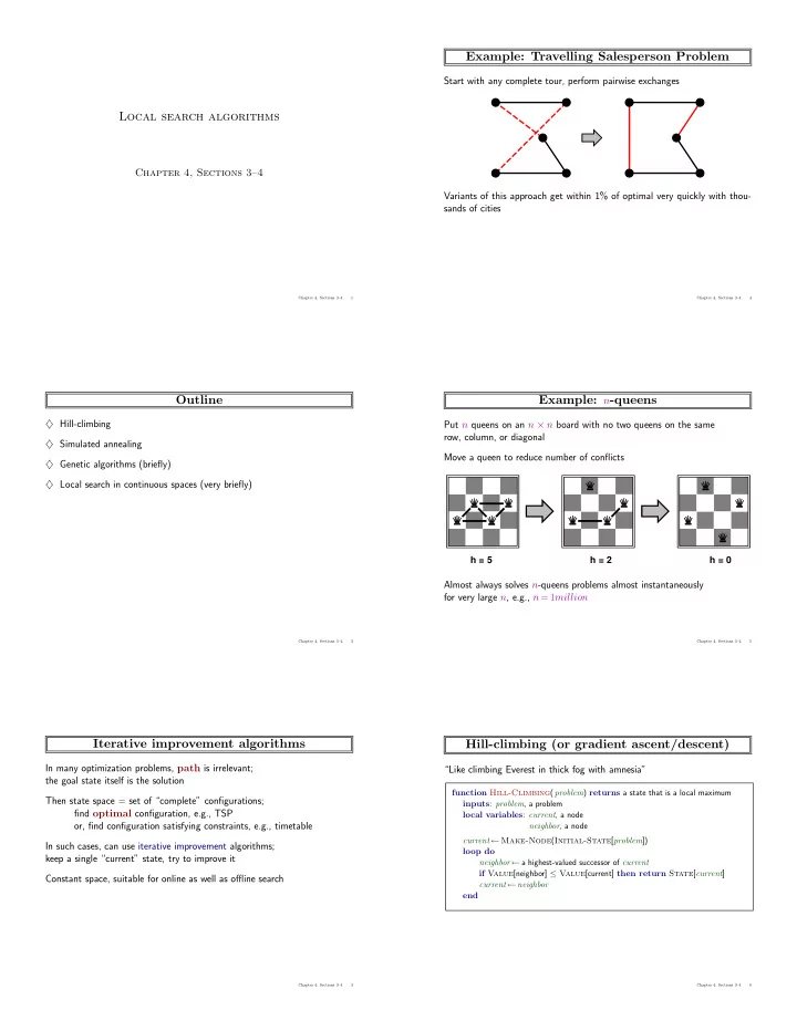current ← neighbor end Chapter 4, Sections 3–4 3 Chapter 4, Sections 3–4 6

Hill-climbing contd. Local beam search Useful to consider state space landscape Idea: keep k states instead of 1; choose top k of all their successors objective function global maximum Not the same as k searches run in parallel! Searches that find good states recruit other searches to join them shoulder Problem: quite often, all k states end up on same local hill local maximum Idea: choose k successors randomly, biased towards good ones "flat" local maximum Observe the close analogy to natural selection! state space current state Random-restart hill climbing overcomes local maxima—trivially complete Random sideways moves escape from shoulders loop on flat maxima Chapter 4, Sections 3–4 7 Chapter 4, Sections 3–4 10 Simulated annealing Genetic algorithms Idea: escape local maxima by allowing some “bad” moves = stochastic local beam search + generate successors from pairs of states but gradually decrease their size and frequency 24748552 24 32748552 32748152 31% 32752411 function Simulated-Annealing ( problem, schedule ) returns a solution state 23 24752411 24752411 32752411 29% 24748552 inputs : problem , a problem 20 32752124 32252124 schedule , a mapping from time to “temperature” 24415124 26% 32752411 local variables : current , a node 24415411 24415417 32543213 11 14% 24415124 next , a node T , a “temperature” controlling prob. of downward steps Fitness Selection Pairs Cross−Over Mutation current ← Make-Node ( Initial-State [ problem ]) for t ← 1 to ∞ do T ← schedule [ t ] if T = 0 then return current next ← a randomly selected successor of current ∆ E ← Value [ next ] – Value [ current ] if ∆ E > 0 then current ← next else current ← next only with probability e ∆ E/T Chapter 4, Sections 3–4 8 Chapter 4, Sections 3–4 11 Properties of simulated annealing Genetic algorithms contd. At fixed “temperature” T , state occupation probability reaches GAs require states encoded as strings (GPs use programs) Boltzman distribution Crossover helps iff substrings are meaningful components E ( x ) p ( x ) = αe kT T decreased slowly enough = ⇒ always reach best state x ∗ E ( x ∗ ) E ( x ) E ( x ∗ ) − E ( x ) kT /e kT = e because e ≫ 1 for small T kT + = Is this necessarily an interesting guarantee?? Devised by Metropolis et al., 1953, for physical process modelling Widely used in VLSI layout, airline scheduling, etc. GAs � = evolution: e.g., real genes encode replication machinery! Chapter 4, Sections 3–4 9 Chapter 4, Sections 3–4 12

Continuous state spaces Suppose we want to site three airports in Romania: – 6-D state space defined by ( x 1 , y 2 ) , ( x 2 , y 2 ) , ( x 3 , y 3 ) – objective function f ( x 1 , y 2 , x 2 , y 2 , x 3 , y 3 ) = sum of squared distances from each city to nearest airport Discretization methods turn continuous space into discrete space, e.g., empirical gradient considers ± δ change in each coordinate Gradient methods compute  ∂f , ∂f , ∂f , ∂f , ∂f , ∂f   ∇ f =     ∂x 1 ∂y 1 ∂x 2 ∂y 2 ∂x 3 ∂y 3  to increase/reduce f , e.g., by x ← x + α ∇ f ( x ) Sometimes can solve for ∇ f ( x ) = 0 exactly (e.g., with one city). Newton–Raphson (1664, 1690) iterates x ← x − H − 1 f ( x ) ∇ f ( x ) to solve ∇ f ( x ) = 0 , where H ij = ∂ 2 f/∂x i ∂x j Chapter 4, Sections 3–4 13