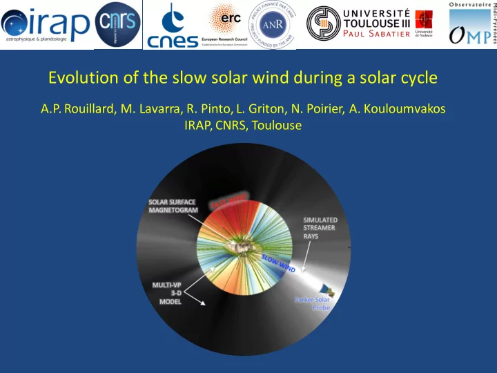
Evolution of the slow solar wind during a solar cycle A.P. - - PowerPoint PPT Presentation

Evolution of the slow solar wind during a solar cycle

A.P. Rouillard, M. Lavarra, R. Pinto, L. Griton, N. Poirier, A. Kouloumvakos IRAP, CNRS, Toulouse

While it is certain that the fast solar wind originates from coronal holes, where and how the slow solar wind (SSW) is formed remains an outstanding question in solar physics.

Several possible origins:

• > the slow wind forms like the fast wind along open field lines!
• > the slow wind forms via continual plasma exchanges between the
• pen and closed corona
• > a component certainly forms via transient releases at the tip of

streamers

The slow wind is a messy story!

Outline

• Intro on slow solar wind and implication for long-

term evolution of the slow wind

• State-state theories for the origin of the slow wind
• Dynamic theories for the origin of the slow wind

Why should we care about the slow solar wind here?

Rouillard et al. 2007 See also : Cliver et al. Mursula et al. 2016

1) There are long-term trends in solar wind properties including solar wind speed:

Wang et al. 2003

2) The slow wind source hosts most of the emergence and shedding

• f open flux over different timescales:

Lockwood et al. 2013

3) The slow wind is likely to hosts CME propagation and very strong particle acceleration

Rouillard et al. 2016 Kouloumvakos et al. 2019

High-energy particles produced near the tip of streamers

4) Lots of fascinating MHD instabilities, kinetic physics and wave- particle interaction to study heating rate and composition of the slow wind.

Laming et al. 2009 Wedemeyer-Bohm et al. 2008

Ko et al. 2018

McComas et al. 2008

FAST WIND

Abbo et al. 2010

Contrasting the origins of slow and fast solar winds:

Differnetial ion heating is weaker in the source region of the slow wind:

Abbo et al. 2013

But temperature anisotropy is therefore also found in the streamer edges and coronal hole boundaries with values in the range of 1.3-2 (Frazin et al, 2003; Susino et al, 2008).

• > Alfvén wave driven solar wind models highly popular

The source region of the slow solar wind has hot electrons!

The ionic charge states are largely fixed in the inner corona (generally below 10Rs), as opposed to density and temperature which change dynamically during the transit in the heliosphere.

Ko et al. 2014

Solar wind ionization states in both fast and slow wind decrease during the declining phase of cycle 23, which should be in some way related to the decreasing solar magnetic field:

• > less magnetic energy would be available to power the wind (Schwadron et al,

2011).

Abbo et al. 2016 Ko et al (2014)

Long-term temperature decrease at the source of the wind:

Abbo et al. 2015

Slow solar wind from unipolar streamers:

• > pseudo-streamers produce a ”hybrid” type of outflow that is

intermediate between slow and fast solar wind and they are apossible source of slow/fast wind in not dipolar solar magnetic field configuration.

Abbo et al. 2015

Slow solar wind from unipolar streamers:

Wang and Sheeley 1990, 1991, 1994, Wang et al. 2008

Flux expansion factor theory:

Basic ingredients to model a ‘realistic’ solar wind:

• suppose the simplest single fluid model with an isotropic distribution function

to reproduce (roughly!) coronal temperatures and solar wind moments:

Transition region Network Network Strongly collisional Partially ionised Weakly collisional Fully ionised Electrons Protons

Ingredients: Anisotropic thermal conduction (extra term or can be included by solving for electrons), Radiative cooling (usually a function), Some heating (choose your favourite!) + an unknown additional contribution to momentum (wave pressure?, electric fields?)

• > V,T,N compare reasonably well with
• bservations.

Hansteen et al.1996, Cranmer et al. 2007, Verdini and Velli 2007, Downs et al. 2009, Lionello et al. 2009)

Photosphere to corona solar wind models run with realistic thermodynamics and high- resolution magneto-static models (PFSS, NLFF):

PFSS (or NLFF) 3-D solar wind plasma

Pinto and Rouillard (2017)

Synthetic imagery SOHO C2

Done by MHD modellers on smoothed magnetograms:

To compare simulations with remote-sensing observations

• We need ‘Realistic magnetic fields’
• To fill in the 3-D volume inside our instruments’ field of view

Pinto and Rouillard 2017

• > Provides space-weather forecasts

3-D (MULTI-TUBE), 1-D flows

Van der Holst 2014 Lionello et al. 2009, Downs et al. 2009 Reville et al. 2018

Full 3-D MHD

AWSoM is awesome!

• Wide-Field Imager : 13.5º - 105º from the Sun.
• Visible Light Observations.
• Next-Generation 2k x 2k APS Sensor.
• Smallest Heliospheric Imager to-date.
• Heritage: STEREO/HI, Solar Orbiter/SoloHI

See PSP Nature special issue (Nov 2019) to evaluate our predictions.

IRAP MHD model prediction for Parker Solar Probe

Michican Ionisation Code (MIC, Landi and co-workers) + AWSoM 3-D MHD (Oran et al. 2015):

• Reproduces the relative charge states of the slow and fast winds,
• Emissions of different ions difficult to re-produce,
• Excursions from average charge state are not explained (footpoint exchange?)
• > supra-thermal electrons (3MK) improve the agreement between observed and

synthetic fluxes of 10 emission lines considered here.

MHD simulations cannot explain both source temperature and brightness of the corona

Geiss et al. 1996

FAST WIND FAST WIND SLOW WIND SLOW WIND

IN SITU DATA

FIP effect

Weak FIP effect Weak FIP effect

Can we model the composition of the solar wind? How do we address the FIP effect?

Kasper et al. 2007

Slow and fast solar winds are very different!

No model is yet capable of simulating coronal composition in 3-D!

On M-stars= Opposite abundance anomaly to solar slow wind and loops.

SLOW WIND SLOW WIND

• 4 x photospheric Fe/O abundance ratio
• Depleted He abundance
• Small proton T anisotropy
• High iron charge states
• Intermittent structures

(see Rouillard et al. 2010, 2011) FAST WIND FAST WIND

• Photospheric Fe/O and He abundance ratio
• Large proton T anisotropy
• Low carbon and oxygen charge states

Fisk (1996)

The slow wind forms along flux tubes that are adjacent and likely to interact with closed loops:

Wang, Nash, Sheeley (late 80s)

e.g. Elephant trunk

Antiochos et al. 2008

Rigid rotation

• f coronal holes

Fisk field S-Web

Can we find signatures of this release process in remote-sensing? Scales, scales, scales ...

Rouillard et al. 2019

COR-2A COR-2B

Arc-like structures emitted over 20-40 degrees PA range 2-3 edge-on blobs per day Sheeley et al. 2008

SIR/CIR

High-speed stream Low-speed stream Low-speed stream High-speed stream

Rouillard et al. (2011a)

High-speed stream Low-speed stream

ST-B If blobs are produced high up in the corona and are flux ropes then can we detect inward motions (i.e. analogous to the SADs in EUV)?

Plotnikov et al. (2016)

Owens and Lockwood 2012 Sheeley and Wang 2001 Sheeley and Wang 2014

Sanchez-Diaz et al. 2016 The release of many blobs had inflows associated with them.

Sanchez-Diaz et al. 2017bc

• > Analysis of in situ data: Sanchez-Diaz et al. 2019

It was estimated that this up owing plasma could form around 25% of the SSW (Harra 2008) However! Considering the small field of view of Hinode/EIS, it is challenging to make a direct link to the solar wind and therefore to determine whether these up flows actually become out flows leaving the Sun. Harra et al. 2008

Upflows are seen by Hinode on the edges of active regions

DeForest et al. 2018

What about far from the current sheet?

Analysis of the near-Earth solar wind during the period 1998–2011 reveals that inverted HMF is present approximately 5.5% of thetime and is generally associated with slow, dense solar wind and relatively weak HMF intensity. Inverted HMF is mapped to the coronal source surface -> a strong association with bipolar streamers containing the heliospheric current sheet, as expected, but also with unipolar or pseudostreamers, which contain no current sheet. Owens et al. 2013

Stay tuned to PSP results!

Quasi steady-state vs Dynamic

EXTRACTION EXPULSION (into wind)

Composition Ionisation states Temperature anisotropies

Diagnostics

(Spectroscopy/In situ)

Multi-species model (H, e-, He, Fe, C, O) Coupling of photo/collisional ionization Include elements of kinetic plasma physics

Magnetic Reconnection (nanoflares?)

Corona Chromosphere

Solar Wind Solar Wind

Transition region Network Network Strongly collisional Partially ionised Weakly collisional Fully ionised

SSW

Electrons Protons Minor ions

CHROMOSPHERIC PHYSICS NON-LTE processes (radiative transfer)

(PhD-1)

CORONAL PHYSICS (plasma/wave transport/heating, non-thermal tails)

(Postdoc-1)

A unique approach at modelling the 3-D multi-species anisotropic corona!

2Mm

Alfvén surface

5 Rs

Kinetic-Fluid solver

Lavarra, Rouillard et al. (In Prep. 2018)

First 3-D multi-species corona

(PhD-1, Postdoc-1, Postdoc-3)

Testing static origin of slow solar wind

Transition region Network Network Strongly collisional Partially ionised Weakly collisional Fully ionised

SSW

Electrons Protons Minor ions

First dynamic multi- species model of corona

Couple to 2.5-D MHD (PhD-2, Postdoc-3) Couple to 3-D MHD (Postdoc-2) (Based on 2.5-MHD: Pinto, Rouillard 2016)

Testing dynamic origin of slow solar wind

Testing the dynamic origin of the slow solar wind!

2Mm

Alfvén surface

5 Rs

How variable is the slow wind composition?

Merci!