SLIDE 1 1 A preliminary version, 11th November 2002. Please do not cite.
Equilibrium Exchange Rates in Transition Countries: Evidence from Dynamic Heterogeneous Panel Models
Byung-Yeon Kim*+ (University of Essex) and Iikka Korhonen (BOFIT) Abstract: We use a dynamic heterogeneous panel model, namely, pooled mean group estimator, to estimate real equilibrium exchange rates for advanced transition
- countries. Our method is based on out-of-sample estimations using middle-income
and high-income countries. We find that in all the five transition countries, the Czech Republic, Hungary, Poland, Slovakia, and Slovenia, exchange rates have converged to real equilibrium exchange rates expressed in the US dollars in recent years. However, we find that the currencies of the countries are substantially overvalued when real effective exchange rates are used. Keywords: exchange rates, transition economies, dynamic heterogeneous panel estimations JEL Classification: C33, F31, P27
* B-Y Kim, Department of Economics, University of Essex, Wivenhoe Park, Colchester CO4 3SQ, United Kingdom. Tel: 44-1206-872777. Fax: 44-1206-872724. E-mail: bykim@essex.ac.uk Iikka Korhonen, Bank of Finland, Institute for Economies in Transition (BOFIT), PO-Box 160, Helsinki, FIN-00101, Finland. E-mail: iikka.korhonen@bof.fi
+We would like to thank for valuable comments participants of an internal BOFIT seminar in
September 2001 and of the BOFIT workshop in April 2002. We would especially like to thank Kari Heimonen and Zsolt Darvas for their comments. Usual disclaimer applies. Part of this research was undertaken while B-Y Kim was visiting BOFIT in 2001. B-Y Kim gratefully acknowledges the excellent research environment offered by BOFIT.
SLIDE 2 2
1. Introduction
Following very high inflation in the early period of transition toward a market economy, stabilisation has already been achieved for most of the advanced transition
- countries. Annual inflation rates in these countries are in single digits, although still
higher than in the European Union (EU). Now new challenges await them. Within a few years, these countries are likely to become EU members. Membership in the EU
- bviously provides new opportunities and benefits for these countries, but it also
imposes a number of obligations. One of these obligations is to become a member of the monetary union, that is, to adopt the euro. In order to satisfy the criterion on exchange rate stability for adopting the single currency, a candidate country must be a member of the Exchange Rate Mechanism 2 (ERM2), which allows the domestic currency to fluctuate within the band of 15% around the central parity, for at least two years without a devaluation of the central parity. Some questions naturally arise in these circumstances. What is the appropriate level of the exchange rate? How can the current exchange rate be evaluated against this appropriate level? Joining first the ERM2 and then euro at an overvalued level of currency suggests loss of competitiveness and subsequently a slower convergence of real incomes towards the EU level. A slow convergence induces cost not only for the transition economics but also for the existing member of the EU through various funds supporting the real convergence within the EU. For example, in 2001 the per capita GDP (calculated with purchasing power adjusted exchange rates) in the accession countries of the Central and Eastern Europe varies from 25% (Romania) to 69% (Slovenia) of the EU average (Eurostat, 2002). In the largest accession country,
SLIDE 3 3 Poland, per capita GDP is 39% of the EU average. Moreover, an overvalued currency is more likely to suffer from a speculative attack. On the other hand, joining the ERM2 with an undervalued exchange rate will result in inflationary pressures. As the exchange rate is fixed, the expected real appreciation of the currency can only take place through higher inflation. This means an increase in the probability of failing the Maastricht convergence criterion on inflation at the ERM2 stage, therefore jeopardising a quick entry into the common currency. Estimating an equilibrium exchange rate in a transition country is not an easy
- task. Main problems include the brief history of the transition period together with
difficulties associated with using data from the socialism period. The socialism period is of little use to estimate an equilibrium exchange rate because prices in a socialist economy failed to reflect an underlying market mechanism. Using data from the transition period, which has lasted for about ten years, is not expected to provide reliable estimation results of an equilibrium exchange rate, because of its short time
- profile. Furthermore, exchange rates during initial transition years were affected
largely by non-conventional factors such as a sharp increase in demand for foreign goods and assets, high expected inflation and the tendency of the authorities to set initial exchange rates at a sharply undervalued level (Halpern and Wyplosz, 1996; Coricelli and Jazbec, 2001). This suggests that a benchmark value for the real exchange rate is misleading particularly for an early period of the transition if data from transition countries are used to estimate equilibrium exchange rates. A more promising approach appears to use an out-of-sample estimation. Several existing studies use the samples of non-transition economies to estimate equilibrium exchange rates in transition countries (Halpern and Wyplosz, 1996; Krajnyák and Zettelmeyer, 1998, Begg et al., 1999). They use dollar wages in a
SLIDE 4 4 sample of (mainly) non-transition countries as proxy for the real exchange rate, and regress dollar wages on a set of variables. Based on the coefficients estimated from the regressions, equilibrium dollar wages are computed for transition countries. All studies find that the initial undervaluation of the real exchange rates was followed by considerable real appreciation, although the currencies of the most transition countries were still undervalued at the end of the sample period. Unfortunately their estimations do not go beyond 1997. This paper analyses an equilibrium exchange rate for five advanced transition countries, namely Poland, Hungary, Czech Republic, Slovenia and Slovakia. We improve on the previous studies by exploiting a time-series and panel dimension of the data set. More specifically, we use a dynamic heterogeneous non-stationary model, Pooled Mean Group (PMG) estimator developed by Pesaran et al. (1996, 1999), and apply this model to real exchange rates against the US dollar of 29 middle- and high-income countries from 1975 to 1999. We also use the sample of 19 middle- and high-income countries from 1980 to 1999 to estimate real effective exchange
- rates. This model allows us to take previous overlooked estimation problems into
account: non-stationarity of the data, heterogeneity across countries, dynamics, and differentiation between long-run and short-run properties. Based on PMG estimation results, we calculate equilibrium exchange rates for the sample countries, and then apply the resulting coefficients to compute the equilibrium exchange rates for the transition countries. These equilibrium exchange rates are, in turn, compared with the actual exchange rates, allowing us to assess the degree of over- or undervaluation. We also perform robustness checks on our results. The paper is structured as follows. Section 2 reviews literature on exchange rates in transition economies. Section 3 discusses our methodology. Following a brief
SLIDE 5 5 discussion on our data set and model, Section 4 presents estimation results of long-run equilibrium exchange rates, and evaluates misalignment of the actual exchange rates in transition countries. Section 5 checks robustness of our results with some alternative estimations of equilibrium exchange rates. Section 6 concludes.
2. Real exchange rates in transition economies
Exchange rate has been one of the central policy tools for many transition economies to stabilise their economy. Transition countries have adopted diverse exchange rate
- regimes. Some have opted for a very hard version of peg, i.e. currency board, while
- thers have adopted a more conventional fixed exchange rate regime or managed
- floating. Most of the countries have changed course along the way in response to
different economic circumstances. Despite of the diversity of exchange rate regimes, these countries in general share a common trend of exchange rate movements. Usually, a sharp initial nominal and real depreciation of currency was followed by real appreciation as domestic inflation exceeded subsequent nominal depreciation and foreign inflation over the course of transition. In this section we first review briefly the relevant literature on the determinants of equilibrium real exchange rates, and then focus on studies concerning real exchange rates in transition countries. 2.1 Determinants of equilibrium real exchange rate Real exchange rate (RER) is generally defined as the nominal exchange rate adjusted for price level differences between countries. More formally, denote RERt as the real exchange rate (in period t), Et as the nominal exchange rate (in units of foreign
SLIDE 6 6 currency per one unit of domestic currency), Pt as the domestic price level and Pt* as price level in the foreign country. RER can be expressed as:
t t t t
P E P RER
*
According to our definition, increase in real exchange rate index means depreciation. In our empirical application, we first look at the bilateral real exchange rate of sample countries vis-à-vis United States. Another exchange rate we consider is the real effective exchange rate (REER), which is a weighted real exchange rate index. The REER is calculated as a weighted average of individual bilateral real exchange rates, and the weights used are the shares of different countries in the home country's foreign trade. MacDonald (1999) lists factors that are likely to determine movements in the real exchange rate. Note that price levels Pt and
* t
P in equation (1) can be decomposed into separate price indices for traded and non-traded goods, and denote price index for traded goods with superscript T and price index for non-traded goods with superscript NT. By taking logarithms of (1) and decomposing prices into traded and non-traded goods, we obtain: ) ( ) (
* * * * NT t T t NT t T t T t t T t t
p p p p p e p rer
where and
*
are the shares of non-traded goods in the overall price index in the home and foreign country, respectively, and small letters denote to logarithms of the variables. There are a number of studies discussing the determinants of equilibrium exchange rates (see, e.g., Baffes et al., 1999; Edwards, 1989, 1994; Montiel, 1999). According to Montiel (1999), the long-run equilibrium real exchange rate emerges
SLIDE 7 7 from macroeconomic equilibrium in an economy when policy and exogenous variables are sustainable in the long-run. He suggests the following set of variables that might be associated with the long-run equilibrium real exchange rate. First, domestic supply-side factors, in particular, the variables relating to the Balassa- Samuelson effect, which arises from faster growth in productivity in the traded-goods sector than in non-traded goods sector, should be considered. The Balassa-Samuelson theorem presupposes that the purchasing power parity (PPP) applies to the market for traded goods (i.e.
T t t T t
p e p
is constant), but the ratio of traded to non-traded goods’ prices may develop differently in different countries. More specifically, in poorer countries the potential for productivity growth in the traded sector is higher than in the more affluent countries, i.e. poorer countries tend to grow faster than richer ones, ceteris paribus. It is also assumed that productivity in the non-traded sector rises more slowly, but real wages are the same in both sectors. Then the real exchange rate appreciates in the country with faster growth rate, even if the PPP holds for the traded sector. Second, fiscal policy measures such as changes in the composition of government spending between traded goods and non-traded goods may affect the equilibrium exchange rate. Such demand side bias affects the real exchange rate as
- follows. If the income elasticity of non-traded goods is larger than unity, their relative
price will rise in tandem with living standards, and consequently the real exchange rate will appreciate. Also, if government expenditure is more geared towards non- traded than traded goods (which is probably a good approximation of reality, since many public services are quite labour-intensive), and the share of government expenditure increases over time, the demand bias may increase an actual real exchange rate.
SLIDE 8 8 Other proposed factors that are associated with long-run equilibrium exchange rates include changes in the international economic environment including terms of trade, the availability of external transfers, and commercial policy like trade liberalisation. 2.2 Real exchange rates in transition countries Using the monthly dollar wage as a proxy for the real exchange rate, Halpern and Wyplosz (1997) estimate first the equilibrium dollar wage for eighty countries and then apply the obtained coefficients to calculate equilibrium dollar wages for a group
- f transition countries between 1991 and 1996. They find that the equilibrium dollar
wages (i.e. equilibrium real exchange rates) had increased in all countries throughout the period in question. Moreover, they imply that by 1996, the real exchange rate is near to its equilibrium level for the Czech Republic, Poland, Slovenia and Hungary. Krajnyák and Zettelmeyer (1998) use a similar methodology as in Halpern and Wyplosz (1996) to estimate the equilibrium dollar wages of fifteen transition countries from 1990 to 1995. They find that the dollar wages were initially lower than the equilibrium wages, but this gap had decreased somewhat by 1995, although not
- completely. In addition, they suggest that the equilibrium wages were rising in Central
and Eastern European countries, while they were more or less flat in former Soviet
- republics. In Begg et al. (1999) a similar analysis to Halpern and Wyplosz (1996) was
extended to more transition countries with the year 1997 added. The basic insights
- ffered by Halpern and Wyplosz (1996) remain valid also in the extended framework.
In particular, according to estimation results, the currencies of the Czech Republic and Slovakia were in line with their equilibrium level, while those of Hungary, Poland and Slovenia were close to overvaluation from 1996 on.
SLIDE 9
9 De Broeck and Sløk (2001) analyse the determinants of real effective exchange rates in 26 transition countries between 1993 and 1998. First they note that almost all countries have experienced clear appreciation of their real effective exchange rate. By 1998 the relationship between per capita GDP and the ratio of purchasing power parity-based and nominal USD dollar exchange rate was broadly similar in transition countries than in a sample of 149 countries. Therefore the initial undervaluation of the currencies had more or less vanished. Coricelli and Jazbec (2001) study determinants of real exchange rates in a wide variety of transition economies. Their proxy for real exchange rate is the relative price of tradable goods in a given country, which allows a direct analysis of the effects of productivity changes on the real exchange rate. Productivity changes, or at least potential for productivity changes, are large in most transition countries. They find that not only more conventional variables but also the variable relating to structural reforms (i.e. the ratio of people employed in industry to those employed in services) are highly significant. A higher share of people working in industry (reflecting lower level of structural reforms) depreciates the real exchange rate. Therefore, the authors conclude that in transition countries structural reforms can have a substantial effect on real exchange rate, over and above the effects that realise through the normal Balassa-Samuelson channel.
3. Dynamic heterogeneous panel model
Most cross-country studies with time dimension have estimated equilibrium exchange rates using pooled OLS or static fixed-effects regressions. However, this traditional approach has several problems. First, it is well known that non-stationarity
SLIDE 10 10
- f the data will lead to spurious regressions if a simple fixed effect model or a pooled
OLS is applied (Pesaran et al., 1996; 1999).1 Second, dynamic properties of the model are overlooked. Clearly, determination of exchange rates is a dynamic process and static specifications are unlikely to capture essential features of such processes. Third, the discussion on the determinants of the equilibrium exchange rate is meaningful
- nly when one can differentiate long-run from short-run parameters. Unless short-run
responses are abstracted, the estimation of parameters of interest can be contaminated, violating conclusions drawn about the importance of factors in determining equilibrium exchange rates. Yet, overlooked non-stationarity of the data, neglected dynamics and possible heterogeneity of short-run responses are frequent problems faced by applied work. We investigate an estimator that takes account of the above problems in traditional approach: the Pooled Mean Group Estimator (PMG) proposed by Pesaran et al. (1996, 1999). This estimator has been recently applied in various empirical studies (Haque, et al., 2000; Asteriou and Price, 2000; Asteriou, et al., 2000; De Broeck and Sløk, 2001). In PMG estimations, cross-sectional heterogeneity is permitted in short-run responses and intercepts, while long-run relationships are common across the panel. Yet the short-run responses and intercepts can differ across countries, reflecting e.g. the diversity in institutional structures across countries. In
- rder to check the robustness of our results, we also use another heterogeneous
1 Pesaran et al. (1999) suggest that in the presence of dynamics and slope heterogeneity the use of
standard panel techniques, such as the fixed-effects estimator or the Anderson-Hsio estimator, leads to inconsistent estimates and potentially misleading inferences even for large N (the number of countries) and T (the number of time periods) panels. Pesaran and Smith (1995) also show that in the case where T is small under certain assumptions the cross section regression based on time-averages of the variables will provide consistent estimates of the long-run coefficients. However, the required assumptions are quite strong. Only for the special case in which the regressors are strictly exogenous and the dynamics are homogeneous across members of the panel can valid inferences be made from the standardised distribution of a coefficient or its associated t-statistic.
SLIDE 11 11 dynamic panel estimator, Fully Modified Ordinary Least Squares (FMOLS), developed by Pedroni (1997, 1999). The two estimators will provide cointegrating vectors between the variables. The PMG is based on the maximum likelihood estimation while the FMOLS uses a modified OLS as the name suggests. These methods allow researchers to selectively pool information regarding common long-run relationships from across the panel, while allowing the associated short-run dynamics and fixed effects to be heterogeneous across different members of the panel. Additional advantage is that, by allowing data to be pooled in the cross-sectional dimension, non-stationary panel methods have the potential to improve upon limitations of short time series.
4. Estimation of equilibrium exchange rates
Data We use data from 29 middle- and high-income countries from 1975 to 1999. Among the sample countries, 13 countries are classified as middle-income and 16 as high- income countries by the World Bank.2 From the sample of countries whose data are fully available for the variables, we exclude small middle-income countries, which we define as countries with population less than ten million. It is likely that exchange rate movements in these countries are affected by price changes of single export items, causing deviations in the long-run behaviour of their exchange rate compared to other economies.
2 Countries used in estimations are: Algeria, Chile, Colombia, Guatemala, Republic of Korea,
Malaysia, Mexico, Morocco, Philippines, South Africa, Thailand, Turkey, Venezuela, Australia, Austria, Belgium, Canada, Cyprus, France, Greece, Hong Kong, Iceland, Ireland, Italy, Japan, Norway, Portugal, Sweden, Switzerland.
SLIDE 12 12 Some explanations are necessary why we propose to use a sample that comprises of middle-income and high-income countries. The transition economies share similar characteristics both with high- and middle-income countries. Their gross domestic product per capita are similar to the level of middle-income countries: the average per capita GDP in 13 middle-income countries in our sample is around 3500 US dollars in 1998 while the average of four transition countries, namely the Czech Republic, Hungary, Poland, and Slovakia is about 4300 US dollars in the same year. Yet, in terms of industrial and trade structure, they are more similar to high-income
- countries. For example, 72% of exports from Central and Eastern Europe is directed
to developed countries while developing countries export only 59% of their total exports to developed countries in 1999 (United Nations, 2000). Of course, the assumption of the poolability across different countries will be tested within the framework of the PMG estimator. After analysing determinants of real exchange rates in our sample of 29 countries, we use the obtained coefficients to calculate equilibrium exchange rates for the five advanced transition countries. We exclude less advanced transition countries such as former Soviet republics, Romania and Bulgaria, because their brief history and the likely lack of the long-run nature of these countries might make our analysis difficult to apply. In addition, we exclude some small and very open transition countries such as the three Baltic countries. Given their extremely small size and very high degree of openness, our approach would not be suitable to capture equilibrium exchange rates of these countries. Model
SLIDE 13 13 Our model follows the concept of the Behavioural Equilibrium Exchange Rate (BEER). One can expect that the actual real exchange rate is in equilibrium in a behavioural sense when its movements reflect changes in the fundamentals of the economy that are found to be related to the actual real exchange rate in a well-defined statistical manner (Clark and MacDonald, 1998), as was discussed previously. In this approach, the equilibrium exchange rate is directly estimated using an appropriate set
- f explanatory variables, and the long-run relationship between the exchange rate and
explanatory variables is derived and interpreted as the equilibrium exchange rate. Basically we are interested in the following long-run relationship between real exchange rate and the four exogenous variables:
it it it it i it
gov cap gdp rer
4 3 2 1
In (3), rerit is the real exchange rate of the domestic currency in a country i and year t. gdpit is GDP per capita in a country i and year t, as a proxy for the Balassa-Samuelson
- effect. It can also be viewed as the proxy for terms of trade effect.3 capit is investment
represented by the share of gross fixed capital formation as a percentage of GDP in a country i and year t. This is intended to capture the domestic supply capacity and possibly technological progress. govit is defined as the share of government consumption as a percentage of GDP in a country i and year t, which captures the effects of fiscal policy. openit is the degree of openness measured by the share of the sum of the volume of export and import as a percentage of GDP in a country i and
3 In the literature, the variable of the terms of trade is often used to represent changes in the
international economic environment. However, these data are not available for many countries in our sample, so we use instead gdpit by assuming that a rise in terms of trade affects GDP positively.
SLIDE 14 14 year t, which reflects the impact of commercial policy or trade regime.4 Note that the intercept term αi is allowed to differ between countries. We have omitted the dynamic term from equation to make presentation more compact. Estimation results: Real exchange rates We first test whether the variables we use in estimations are non-stationary and estimated equations are actually cointegrated. Therefore we first conduct panel unit root tests suggested by Hadri (2000) for all our variables. Results are reported in Table 1. All test statistics are significantly different from zero and thus the null of stationarity is strongly rejected. Following the identification of the order of integration, we estimate the model (3) using PMG. In these estimations, we use the real exchange rate of the domestic currency relative to the US dollar, as the dependent variable. For comparison, we also report the results of the Mean Group (MG) estimator (i.e. estimations were done separately for each country, and panel coefficients were obtained by averaging over individual country coefficient estimates). The joint Hausman test is used to determine whether common long-run coefficients are applicable to the whole sample. Rejection
- f the test would suggest that the sample is too heterogeneous to be pooled.
Table 2 shows estimation results of the two estimators. The results are fairly similar regarding the sign and size of the coefficients. This is encouraging because the two estimators use different methods to estimate the model. Compared to the results using MG estimator, the PMG results improve the precision of estimations. The comparison between MG and PMG results indicates that imposing long-run homogeneity reduces the standard errors of the long-run coefficients, but does not
4 The data are obtained from the following two sources: IMF, International Financial Statistics; the
SLIDE 15 15 change the estimates very much. This is confirmed by the Hausman test statistic, which suggests the sample countries can be pooled to provide a common long-term coefficients. The estimation results are consistent with theoretical predictions. The Balassa- Samuelson effect, as captured by GDP per capita, appreciates a currency. Increases in capital stock are positively associated with the appreciation of a currency. Roughly speaking, one per cent increase in the per capita GDP is associated with a real appreciation of 0.8%. Increases in the share of government spending also appreciate real exchange rate, suggesting that government spending as the share of GDP goes more to the non-tradable sector than the tradable sector. If government expenditure is more geared towards non-traded than traded goods, a larger share of government expenditure will result in the appreciation of real exchange rate. In contrast, as in
- ther literature, openness depreciates a currency. In terms of the magnitude of the
coefficients, the Balassa-Samuelson effect exerts the largest influence on the real exchange rate, followed by openness, government consumption and capital formation. We apply the coefficients appearing in Table 2 to the sample countries to have a feel about the reliability of our estimates. Note that the deviation of an actual exchange rate from an ‘equilibrium’ exchange rate do not necessarily mean that the currency of a country in our sample is over- or undervalued. In order to determine to what extent the currency deviates from its equilibrium level, we need to use the sample of countries that have similar characteristics. By pooling middle-and high- income countries, equilibrium exchange rates estimated as above are intended to apply to the five transition countries not to sample countries used for our estimation. Our main purpose is first to understand whether the two estimates provide consistent
World Bank, World Development Indicators.
SLIDE 16 16
- results. One can also expect that high-income countries tend to display overvalued
currencies while middle-income countries find that their currencies are undervalued. This is because that by pooling middle-income countries with high-income countries, we disregard a premium associated with high-income countries. Lastly, it is expected that some sample countries whose economic features and performances are similar to the five transition countries would have relatively smaller deviations compared to the
Figure 1 displays the extent of deviations of a currency from an equilibrium level for each country evaluated with common intercept. The horizontal axis refers to the annual average of PPP GDP per capita from 1975 to 1999. Eight middle-income countries out of 13 belong to the group in which their currencies are undervalued while the currencies of 14 high-income countries out of 16 appear to be overvalued. This is in general consistent with our expectation that the currencies of middle-and high-income countries will be undervalued and overvalued respectively if we apply a common intercept across these countries. The average of deviations for the sample countries is –0.226. The figures also imply that transition countries will have a similar intercept as countries such as Ireland, Cyprus, and Turkey have had over the sample
- period. This seems not too unreasonable given the stage of economic development in
both groups of countries. The equilibrium exchange rate for transition economies is computed using the coefficients obtained from the previous estimations. We also apply the common intercept calculated above. Exchange rates are normalised in a way that actual exchange rates in 1995 were set to one. Figures 2-6 show that actual real exchange rates in all the five advanced transition countries have been quite close to equilibrium exchange rates during the
SLIDE 17 17 latter half of the 1990s. With the exceptions of Slovakia and Slovenia, the currencies
- f the other three countries were substantially undervalued during the initial transition
- period. Following the period of undervaluation, there has been a strong tendency for
the real exchange rate to appreciate and to converge closer to its equilibrium value. By 1999, in the four of the five transition countries, actual real exchange rates were in line with equilibrium exchange rates. The only exception was Slovenia: following an exchange rate that was very close to the equilibrium level in 1995, its currency was undervalued in 1999. Paths to achieving convergence varied across the countries. Real appreciation
- f the currencies was a main contributor to the convergence in the Czech Republic,
Hungary, and Poland during the early years of the transition. After that, depreciation in the equilibrium exchange rates, reflecting changes in economic fundamentals (especially openness), became more dominant in achieving the convergence in the Czech Republic and Hungary. In contrast, a continuous appreciation of the real exchange rate in Poland helped to make the zloty more aligned with its equilibrium
- level. The Slovakian currency appears not to have been substantially undervalued at
the initial period of transition. Following the period of a widening gap between the actual exchange rates and the equilibrium rates from 1992 to 1995, the convergence process in Slovakia had started from 1996, displaying the actual rate was broadly in line with the equilibrium rate in 1999. In Slovenia, the real exchange rate was quite stable under the period we study (especially in the second half of the 1990s), reflecting policy-makers’ preference for stability. Another striking finding concerning Slovenia is that her currency appears undervalued substantially from 1997 to 1999, which suggests that the promotion of exports through a weaker domestic currency has been used extensively as an important policy tool in Slovenia.
SLIDE 18 18 In sum, actual real exchange rates measured against the US dollars were more
- r less in line with equilibrium exchange rates in the four advanced transition
countries by the end of 1990s. These results do not differ substantially from the findings of the earlier studies. However, we find that unlike Begg et al., (1999), the currencies of Hungary and Poland are fairly close to its equilibrium level from 1996 to 1999 in terms of real exchange rates. The convergence had been achieved in the Czech Republic, Hungary, Poland, and Slovakia during the period of 1995-1999: Hungary is the first country to had converged to the equilibrium real exchange rate, followed by Poland, Slovakia and the Czech Republic. In contrast, we find evidence that the currency of Slovenia was possibly undervalued in 1999 even by 28%. Estimation results: Real effective exchange rates Now the question is whether the convergence of actual exchange rates to equilibrium exchange rates still holds when we use the real effective exchange rate. Because of limited availability of data on real effective exchange rates, the sample used is reduced to 19 countries, comprising of 7 middle-income countries and 12 high- income countries. This data limitation may cause a bias toward high-income countries, because the share of high-income countries of total sample countries we use for the analysis of real effective exchange rates is higher than that for the investigation
- f real exchange rates. Among the five transition countries, Slovenia is also dropped
from the analysis because of the lack of the necessary data. Table 3 presents estimation results of the two estimators.5 Imposing long-run homogeneity is accepted by the Hausman test statistic, suggesting there is a common long-run cointegration vector. In addition, the sign of the coefficients on the
SLIDE 19 19 explanatory variables are the same as in the previous estimation using USD real exchange rates and across the two estimators. Yet, there are sizable differences in the magnitude of coefficients between PMG and MG estimators, implying that the precision of estimates of equilibrium real effective exchange rates is somewhat compromised. Figure 7 displays average deviations from real effective equilibrium exchange rates in our sample countries. The horizontal axis is the annual average of GDP per capita from 1980 to 1999. According to the figures, the currencies of all middle- income countries are undervalued, while those of high-income countries, apart from Cyprus, are overvalued. The average of deviations from the equilibrium real effective exchange rates is 0.046, which is higher by 0.273 compared with the average of deviations shown in Figure 1. Figure 7 presents that the currency of Cyprus has one of the lowest deviations from the equilibrium level, as in Figure 1. In addition, the two figures suggest similar results in terms of the extent of deviations across countries. Yet, compared to Figure 1, the countries are more widely dispersed.6 In order to estimate the equilibrium level of real effective exchange rates and to facilitate a comparison across the two concepts of exchange rates, we adjust the common intercept in Figure 7 to that of Figure 1. The reason is that a bias toward high- income countries, because of the lack of data on some middle-income countries, is likely to have caused the higher average deviation for real effective exchange rates compared with that of US dollar-based real exchange rates. Note that this adjustment will affect a domestic currency in the direction toward its depreciation.
5 The countries to use in the estimations are: Algeria, Chile, Colombia, Morocco, Philippines, South
Africa, Venezuela, Austria, Belgium, Canada, Cyprus, France, Iceland, Italy, Japan, Norway, Portugal, Sweden, Switzerland. The sample period is from 1980 to 1999.
6 Standard errors of the deviations based on PMG appearing in Figures 1 and 7 are 0.51 and 0.68,
respectively.
SLIDE 20 20 Figures 8-11 show real effective equilibrium exchange rates compared to actual real effective exchange rates. The most striking feature is that currencies of all four countries, the Czech Republic, Hungary, Poland and Slovakia turn out to be
- vervalued during 1998-99, when real effective exchange rates are applied. The
extent of overvaluation differs across countries. The currencies of Poland and Slovakia appear to be overvalued by about 8%, followed by the Czech Republic whose currency is overvalued by 12%. Furthermore, Figure 9 suggests that the Hungarian currency is overvalued by more than 40%. Although the Hungarian currency was undervalued by 15% in 1990, sharp depreciation in equilibrium exchange rate particularly from 1994 to 1998 together with real appreciation of real effective exchange rate seem to have widened the gap between equilibrium exchange rates and actual exchange rates. Real equilibrium exchange rates at the beginning of transition were likely to be affected by several short-term factors including transitional recession, CMEA trade, etc. (Dibooglu, 2001; Coricelli and Jazbec, 2001). As regards the Hungarian currency, one of the reasons why her currency appears to be overvalued might be large capital inflows including foreign direct investment (FDI) into Hungary. For example, Hungary has received average annual net FDI inflows of 5% of GDP during the 1990s, while the share of FDI inflows for the Czech Republic, Poland and Slovakia were 3.5%, 2.4%, and 1.7% of GDP, respectively, during the same period. If the level of capital inflows in Hungary is not sustainable in the long-run, the Hungarian currency could depreciate closer to the level determined by fundamentals. A comparison between equilibrium exchange rates and actual ones should be taken very cautiously. Although one would expect that long-term factors become more important over time, it is still not so clear that the movements of variables in
SLIDE 21 21 these countries reflects long-run steady states. All in all, one should not expect that the equilibrium exchange rate is known with any degree of precision. With some reliability, however, our exercise provides information on the extent of deviations from the equilibrium levels, and perhaps with more reliability, on whether the currencies of these countries are under- or overvalued. Looking at our estimates for long-run coefficients, we may learn the reasons for very different conclusions regarding over- or undervaluation of currencies when using USD-based real exchange rate and real effective exchange rate. Openness depreciates the equilibrium exchange rate less compared to the case in which estimates are done with real effective exchange rates. As the transition countries we focus on are quite open, this has an influence on the calculated equilibrium exchange
- rate. Furthermore, when estimations are conducted with US dollar-based real
exchange rates, per capita GDP has clearly larger influence on the equilibrium exchange rate than the case in which the estimations are based on real effective exchange rates (with US dollar-based estimations per capita GDP appreciates more the equilibrium exchange rate). One of the most plausible explanations appears that the main trade partners of these countries are members of the European Union, whose currencies were most probably significantly undervalued against the US dollar during the latter half of
- 1990s. The findings suggest that currencies of the transition countries are well aligned
with their equilibrium level in terms of USD real exchange rates but not anymore in terms of real effective exchange rates: they might be substantially overvalued against EU currencies. This would fit in with the finding that the currencies of the EU countries on average were undervalued by 15-20% against the US dollar at the end of 1999 (Alberola et al., 1999).
SLIDE 22 22
5. Robustness checks
We check the robustness of our results in two ways. First, we employ a different estimator to estimate real (effective) equilibrium exchange rates. This can be viewed as a test how sensitive the results are depending upon using a different estimation
- method. Second, in order to calculate equilibrium exchange rates, we apply different
intercepts that reflect some heterogeneity within the transition countries. Different estimator We use the Fully Modified OLS (FMOLS) proposed and applied by Pedroni (1995, 1999). As with the PMG, FMOLS allows very general degree of cross-sectional heterogeneity in short-run responses and intercepts, but long-run relationships are set to be common across the panel. Yet, unlike the PMG that uses maximum likelihood method, FMOLS is based on modified OLS. Table 5 suggests that estimation results based on PMG appearing in Table 2 are largely robust. All the coefficients obtained by applying FMOLS have the same signs and similar magnitudes as the previous PMG results, suggesting equilibrium real exchange rates derived from the PMG method are roughly equal to those from
- FMOLS. The comparison of results in Table 6 with those in Table 3 indicates that
there are some differences in the magnitude of coefficients. However, applying coefficients derived from FMOLS to data from the transition countries does not affect the extent of overvaluation of the currencies substantially: when FMOLS is applied, the Czech currency appears to be overvalued by 13%, the Hungarian currency by 44%, the Polish one by 13%, and the Slovakian one by 8%. Different intercepts
SLIDE 23 23 Previously we applied the common intercept to the all five transition economies to derive equilibrium exchange rates. Yet, one can argue that there is some heterogeneity across these countries that may affect equilibrium exchange rates. We allow the role
- f such heterogeneity in determining equilibrium exchange rates by assuming that the
level of economic development in a country is the main determinant of heterogeneity. We use GDP per capita as a proxy of the level of economic development in a country. We first regress deviations of actual exchange rates from equilibrium exchange rates appearing in Figures 1 and 7 on GDP per capita in each country. Using the coefficient on the regressor, we calculate an intercept for each of the five transition countries. Since the average of GDP per capita of sample countries is higher than that of the transition countries except Slovenia from 1992 to 1999, it is expected that applying this method contributes to depreciating the equilibrium real exchange rate in these countries except Slovenia from 1992 to 1999. Table 7 shows equilibrium exchange rates of the transition countries in 1999 with having a common intercept and a different intercept, respectively. Although there are some changes in the extent of misalignment, the basic findings remain the
- same. With the exception of Slovenia, currencies of all other transition countries are
in line with the US dollar-based real equilibrium exchange rates. However, when the real effective exchange rates were used, these currencies turned out to be overvalued. Applying a different intercept suggests that they are undervalued by about 20 percent for the Czech Republic, Poland and Slovakia, and by 49 percent for Hungary.
6. Conclusions
We use dynamic panel heterogeneous models to estimate real and real effective equilibrium exchange rates in advanced transition countries. Our estimation method
SLIDE 24 24 rates is based on out-of-sample estimations using middle-income and high-income
- countries. We apply PMG estimator developed by Pesaran et al. (1996, 1999) to our
sample of countries. Coefficients obtained from estimations are applied to derive real equilibrium exchange rates of the transition countries. We find that in all the five transition countries, the Czech Republic, Hungary, Poland, Slovakia and Slovenia, domestic currencies have converged to real equilibrium exchange rates expressed against the US dollar. At the outset of transition process, currencies of these countries were clearly undervalued. Over time, however, there was the process of substantial real appreciation that made the currencies converge to their equilibrium levels by 1999. However, a strikingly different result emerges when we estimate real effective exchange rates. We find that the currencies
- f the Czech Republic, Hungary, Poland and Slovakia are substantially overvalued.
The extent of overvaluation varies ranging between 8% and 40%. This may be explained partly by evidence that the currencies of EU countries, which are main trading partners for the transition countries, are undervalued against the US dollar. Our findings imply that serious challenges lie ahead for the exchange rate policy in EU accession countries. Joining the euro at the current level of exchange rate may undermine export to EU countries and thus catching-up process. Although ERM-2 allows a significant room for fluctuation of a currency against the central parity, highly overvalued currency is more likely to suffer from a currency
- speculation. One possible option to consider is to delay joining the euro area until
there is substantial catching-up resulting from prolonged higher economic growth. Our study should be considered only a tentative step towards estimating equilibrium exchange rates in the accession countries. Estimation results should be taken as approximations, not as precise results. Obviously, more work needs to be
SLIDE 25
25 done to understand different results in equilibrium exchange rates obtained by different methodologies.
References
Alberola, Enrique, Cervero, S., Lopez, Humberto, and Ubide, Angel, (1999), “Global equilibrium exchange rates: euro, dollar, “ins,” “outs,” and other major currencies in a panel cointegration framework,” International Monetary Fund Working Paper 175.
SLIDE 26 26 Asteriou, D., and Price, S, (2000), “Uncertainty, investment, and economic growth: evidence from a dynamic panel, City University. Asteriou, D., Lukacs, P., Pain, N., and Price, S., (2000), “Manufacturing price determination in OECD countries: markups, demand and uncertainty in a dynamic heterogeneous panel, mimeo, City University. Baffes, John, Elbadawi, Ibrahim A. and O'Connell, Stephen A. (1999), “Single- equation estimation of the equilibrium real exchange rate,” In Lawrence E. Hinkle and Peter J. Montiel, Eds., Exchange Rate Misalignment: Concepts and Measurement for Developing Countries.
- Begg. David, Halpern, László, and Wyplosz, Charles, (1999), Monetary and exchange
rate policies, EMU and Central and Eastern Europe. Forum Report of the Economic Policy Initiative, No.5. CEPR. Clark, Peter B. and MacDonald, Ronald, (1998), “Exchange rates and economic fundamentals – a methodological comparison of BEERs and FEERs,” IMF Working Paper 98/67. Coricelli, Fabrizio, and Jazbec, Bostjan, (2001), “Real exchange rate dynamics in transition economies,” CEPR Discussion Paper No.2869. De Broeck, Mark and Sløk, Torsten, (2001), “Interpreting real exchange rate movements in transition countries,” Bank of Finland Institute for Economies in Transition Discussion Paper 7/2001. Dibooglu, Selahattin, (2001), “Sources of real exchange rate fluctuations in transition economies: the case of Poland and Hungary,” Journal of Comparative Economics 29, 257-75. Edwards, Sebastian, (1989), “Real exchange rates in the developing countries: concepts and measurement,” NBER Working Paper, No. 2950.
SLIDE 27 27 Edwards, Sebastian, (1994), “Real and monetary determinants of real exchange rate behavior: theory and evidence from developing countries,” in Estimating Equilibrium Exchange Rates, ed. By Williamson, John, Washington D.C., Institute for International Economics. Eurostat (2002), Statistical yearbook on candidate and South-East European countries. Luxembourg. Hadri, Kaddour (2000), “Testing for stationarity in heterogeneous panel data,” The Econometrics Journal, Vol. 3, pp. 148-161. Halpern, László and Wyplosz, Charles, (1996), “Equilibrium exchange rates in transition economies,” IMF Working Paper 96/125. Haque, Nadeem, Pesaran, Hashem, and Sharma, Sunil, (2000), “Neglected heterogeneity and dynamics in cross-country savings regressions,” In Panel Data Econometrics - Future Direction: Papers in Honour of Professor Pietro
- Balestra. eds. by J. Krishnakumar and E. Ronchetti, Elsevier Science, 2000,
chapter 3, pp.53-82. Im, K.S., Smith, R., and Pesaran, H, (1996), Dynamic linear models for heterogenous
- panels. In The Econometrics of Panel Data (eds) L. Mátyás and P. Sevestre,
chapter 8, pp.145-195, Kluwer Academic Publishers, Dordrecht, Krajnyák, Kornélia and Zettelmeyer, Jeromin, (1997), “Competitiveness in transition economies: what scope for real appreciation?” IMF Working Paper 97/149. MacDonald, Ronald (1999), "What do we really know about real exchange rates?" In Ronald MacDonald and Jerome L. Stein, Eds., Equilibrium Exchange Rates. Boston, Kluwer Academic Publishers. Montiel, Peter (1999), “Determinants of the long-run equilibrium exchange rate: an analytical model”, in Hinkle, Lawrence and Montiel, Peter, eds, Exchange
SLIDE 28 28 Rate Milalignment: Concepts and Measurement for Developing Countries, World Bank, Oxford University Press, Oxford. Pedroni, Peter, (1995), “Panel cointegration; asymptotic and finite sample properties
- f pooled time series tests, with an application to the PPP hypothesis,” Indiana
University Working Papers in Economics, No. 95-013. Pedroni, Peter, (1999), “Critical values for cointegration tests in heterogeneous panels with multiple regressors,” Oxford Bulletin for Economics and Statistics 653- 670. Pesaran, Hashem, Smith, Ron, and Im, K., (1996), “Dynamic linear models for heterogenous panels,” in The Econometrics of Panel Data eds. by L. Mátyás and P. Sevestre, chapter 8, pp.145-195, Kluwer Academic Publishers, Dordrecht. Pesaran, Hashem, Shin, Yongcheol, and Smith, Ron, (1999) “Pooled mean group estimation of dynamic heterogeneous panels”. Journal of the American Statistical Association, vol. 94 pp.621-634. Sarno, Lucio and Taylor, Mark P. (2001) "Purchasing Power Parity and the Real Exchange Rate," CEPR Discussion Paper No.2913. United Nations, (2000), World Economic and Social Survey. Williamson, John (1985) "The Exchange Rate System." Washington D.C., Institute for International Economics.
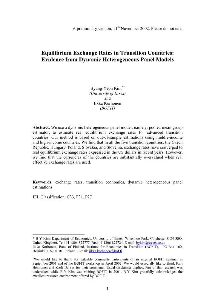
SLIDE 29 29 Figure 1: Deviations from the equilibrium exchange rate in sample countries: (average deviation during 1975-1999) Figure 2: Exchange rates in the Czech Republic
0.2 0.4 0.6 0.8 1 1.2 1.4 1.6 1992 1993 1994 1995 1996 1997 1998 1999 years exchange rates real exchange rates
Philippines Colombia Greece Ireland Japan Switzerland Hong Kong Malaysia
0,5 1 5000 10000 15000 20000 Average GDP per capita, PPP USD Deviation
Morocco Guatemala Thailand Algeria Turkey Venezuela Chile Korea, Rep. South Africa Portugal Cyprus Canada Norway Iceland Belgium Austria Sweden Australia Italy France Mexico
SLIDE 30 30 Figure 3: Exchange rates in Hungary
0.2 0.4 0.6 0.8 1 1.2 1.4 1.6 1990 1991 1992 1993 1994 1995 1996 1997 1998 1999 years exchange rates real exchange rates
Figure 4: Exchange rates in Poland
0.2 0.4 0.6 0.8 1 1.2 1.4 1.6 1.8 1990 1991 1992 1993 1994 1995 1996 1997 1998 1999 years exchange rates real exchange rates
SLIDE 31 31 Figure 5: Exchange rates in Slovakia
0.2 0.4 0.6 0.8 1 1.2 1.4 1.6 1992 1993 1994 1995 1996 1997 1998 1999 years exchange rates real exchange rates
Figure 6: Exchange rates in Slovenia
0.2 0.4 0.6 0.8 1 1.2 1.4 1.6 1991 1992 1993 1994 1995 1996 1997 1998 1999 years exchange rates real exchange rates
SLIDE 32 32 Figure 7: Deviations from real effective equilibrium exchange rate in sample countries: PMG results (average deviation during 1980-1999) Figure 8: Real effective exchange rates in the Czech Republic
0.2 0.4 0.6 0.8 1 1.2 1.4 1990 1991 1992 1993 1994 1995 1996 1997 1998 1999 years exchange rates real effective exchange rates
Philippines
0,5 1 1,5 5000 10000 15000 20000 Average GDP per capita, PPP USD Deviation
Algeria Morocco Colombia Venezuela South Africa Cyprus Switzerland Portugal Japan Italy Sweden France Austria Belgium Canada Norway Iceland Chile
SLIDE 33 33 Figure 9: Real effective exchange rates in Hungary
0.2 0.4 0.6 0.8 1 1.2 1.4 1.6 1990 1991 1992 1993 1994 1995 1996 1997 1998 1999 years exchange rates real effective exchange rates
Figure 10: Real effective exchange rates in Poland
0.5 1 1.5 2 2.5 1990 1991 1992 1993 1994 1995 1996 1997 1998 1999 years exchange rates real effective exchange rates
SLIDE 34 34 Figure 11: Real effective exchange rates in Slovakia
0.2 0.4 0.6 0.8 1 1.2 1.4 1990 1991 1992 1993 1994 1995 1996 1997 1998 1999 years exchange rates real effective exchange rates
SLIDE 35 35 Table 1 Panel Unit Root Tests Hadri’s heterogeneous panel unit root tests* variables test statistic (p-value) rer 2.507(0.006) gdp 4.275 (0.000) cap 2.188 (0.014) gov 2.577 (0.005)
4.441 (0.000)
Notes: These tests perform a Lagrange Multiplier test for stationarity in heterogeneous panel data, suggested by Hadri (2000). The null hypothesis is stationarity. We take two lags and possible serial dependence in the disturbances into account.
Table 2 Long-run Coefficients of Heterogeneous Panel Cointegration Estimations: Real Exchange Rate PMG estimator MG estimator
coefficients t-values coefficients t-values gdp
cap
gov
0.65 22.07 1.01 2.50 error- correction
Joint Hausman Test 1.25 (0.87) Notes: The order of lag was chosen based on the Akaike Information Criterion for PMG and MG
- estimators. The order of lag in most of the countries is either 1 or 2.
SLIDE 36 36 Table 3 Long-run Coefficients of Heterogeneous Panel Cointegration Estimations: Real Effective Exchange Rate PMG estimator MG estimator
coefficients t-values coefficients t-values gdp
cap
gov
0.06 0.15
0.36 41.84 0.65 2.69 error- correction
Joint Hausman Test 2.81 (0.59)
SLIDE 37 37 Table 4 Percentage deviations of actual real exchange rates from equilibrium values
Year Real USD exchange rate Real effective exchange rate Czech Republic 1990
1991
1992
1993
1994
1995
1996
1997
1998
11.7 1999
11.9 Hungary 1990
1991
7.3 1992
11.7 1993
8.2 1994
14.6 1995
24.2 1996
31.3 1997 1.4 37.8 1998 4.6 42.0 1999 0.4 40.7 Poland 1990
1991
1992
1993
1994
1995
1.0 1996
6.8 1997 0.6 8.6 1998 6.9 15.9 1999
8.1 Slovakia 1990
1991
1992
1993 2.0 5.7 1994 7.4 15.4 1995 17.7 17.4 1996 11.4 2.4 1997 6.6 6.2 1998 8.3 2.8 1999
8.4 Slovenia 1991 4.5 1992
1993
1994
1995 0.3 1996
1997
1998
1999
Note: A negative (-) sign implies the currency is undervalued.
SLIDE 38 38 Table 5 Long-run Coefficients of FMOLS Panel Cointegration Estimations: Real Exchange Rate FMOLS estimator
coefficients t-values gdp
cap
gov
0.82 16.68 Note: We used the common lag order of two.
Table 6 Long-run Coefficients of FMOLS Panel Cointegration Estimations: Real Effective Exchange Rate FMOLS estimator
coefficients t-values gdp
cap
gov
1.17
0.61 16.19 Note: We used the common lag order of two.
Table 7 Percentage deviations of actual real exchange rates from equilibrium values
Real USD exchange rate Real effective exchange rate Year Common intercept Different intercept Common intercept Different intercept Czech Republic 1999
11.9 19.0 Hungary 1999 0.4 4.6 40.7 48.9 Poland 1999
1.7 8.1 21.0 Slovak Rep. 1999
2.6 8.4 20.2 Slovenia 1999