Empirical Analysis of SLS Algorithms adapted and extended from - PDF document

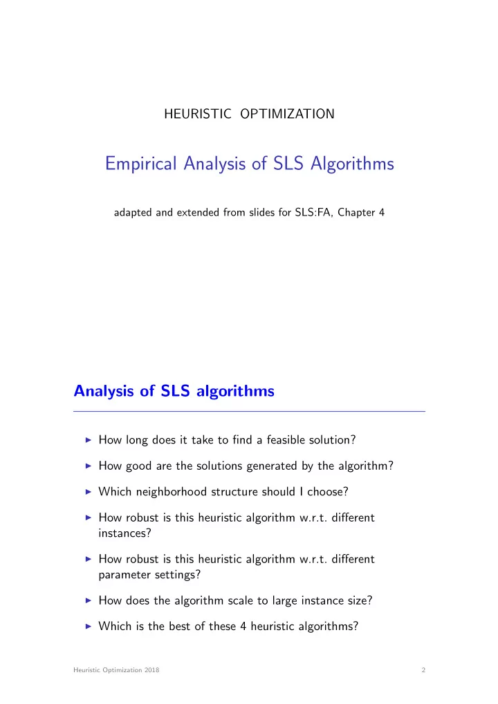
HEURISTIC OPTIMIZATION Empirical Analysis of SLS Algorithms adapted and extended from slides for SLS:FA, Chapter 4 Analysis of SLS algorithms I How long does it take to find a feasible solution? I How good are the solutions generated by the algorithm? I Which neighborhood structure should I choose? I How robust is this heuristic algorithm w.r.t. di ff erent instances? I How robust is this heuristic algorithm w.r.t. di ff erent parameter settings? I How does the algorithm scale to large instance size? I Which is the best of these 4 heuristic algorithms? Heuristic Optimization 2018 2

I ideally: do theoretical analysis, but: I the theoretical analysis of detailed behavior of (advanced) SLS algorithms is often very di ffi cult due to I stochasticity of algorithms I complexity of problems tackled ( NP -hard) I many degrees of freedom in algorithms which make them theoretically hard to capture I practical applicability of theoretical results often limited I rely on idealised assumptions that do not apply in practical situations ( e.g. , convergence results for Simulated Annealing) I capture only asymptotic behaviour and do not reflect actual behaviour with su ffi cient accuracy I apply to worst-case or highly idealised average-case Heuristic Optimization 2018 3 Therefore: Analyse the behaviour of SLS algorithms using sound empirical methodologies Example: follow a scientific procedure: I make observations I formulate hypothesis/hypotheses ( model ) I While not satisfied with model (and deadline not exceeded): 1. design computational experiment to test model 2. conduct computational experiment 3. analyse experimental results 4. revise model based on results Heuristic Optimization 2018 4

Goals of empirical analysis : Obtain insights into algorithmic performance I help assessing suitability for applications I provide basis for comparing algorithms I characterise algorithm behavior I facilitate improvements of algorithms Heuristic Optimization 2018 5 Examine aspects of stochastic search performance I variability due to randomization I robustness w.r.t. parameter settings I robustness across di ff erent instances / instance types I scaling with instance size Heuristic Optimization 2018 6

Run-Time Distributions Empirical analysis of SLS algorithms I traditional approach I run SLS algorithm n times with time limit t max I compute averages, standard deviations I more detailed point of view I for decision SLS algorithms the run time to reach a solution is a random variable (univariate) run-time distributions (RTDs) I for optimisation SLS algorithms the run time and the solution quality returned are random variables (bivariate) run-time distributions (RTDs) study distributions of random variables characterising run-time and solution quality of algorithm on given problem instance. Heuristic Optimization 2018 7 Example of run-time distribution for SLS algorithm applied to hard instance of combinatorial decision problem: 1 0.9 0.8 0.7 P(solve) 0.6 0.5 0.4 0.3 0.2 0.1 0 100 0.001 0.01 0.1 1 10 run-time [CPU sec] Heuristic Optimization 2018 8

Example of run-time distribution for SLS algorithm applied to hard instance of combinatorial decision problem: 1 0.9 0.8 0.7 P(solve) 0.6 0.5 0.4 0.3 0.2 0.1 0 100 0.001 0.01 0.1 1 10 run-time [CPU sec] Heuristic Optimization 2018 9 Example of run-time distribution for SLS algorithm applied to hard instance of combinatorial decision problem: 1 0.9 0.8 0.7 P(solve) 0.6 0.5 0.4 0.3 0.2 0.1 0 100 0.001 0.01 0.1 1 10 run-time [CPU sec] Heuristic Optimization 2018 10

Example of run-time distribution for SLS algorithm applied to hard instance of combinatorial decision problem: 1 0.9 0.8 0.7 P(solve) 0.6 0.5 0.4 0.3 0.2 0.1 0 100 0.001 0.01 0.1 1 10 run-time [CPU sec] Heuristic Optimization 2018 11 Definition: Run-Time Distribution (1) Given SLS algorithm A for decision problem Π : I The success probability P s ( RT A , π  t ) is the probability that A finds a solution for a soluble instance π 2 Π in time  t . I The run-time distribution (RTD) of A on π is the probability distribution of the random variable RT A , π . I The run-time distribution function rtd : R + 7! [0 , 1], defined as rtd ( t ) = P s ( RT A , π  t ), completely characterises the RTD of A on π . Heuristic Optimization 2018 12

Definition: Run-Time Distribution (2) Given SLS algorithm A 0 for optimisation problem Π 0 : I The success probability P s ( RT A 0 , π 0  t , SQ A 0 , π 0  q ) is the probability that A 0 finds a solution for a soluble instance π 0 2 Π 0 of quality  q in time  t . I The run-time distribution (RTD) of A 0 on π 0 is the probability distribution of the bivariate random variable ( RT A 0 , π 0 , SQ A 0 , π 0 ). I The run-time distribution function rtd : R + ⇥ R + 7! [0 , 1], defined as rtd ( t , q ) = P s ( RT A , π  t , SQ A 0 , π 0  q ), completely characterises the RTD of A 0 on π 0 . Heuristic Optimization 2018 13 Example of run-time distribution for SLS algorithm applied to hard instance of combinatorial optimisation problem: P(solve) 1 0.8 0.6 0.4 0.2 0 2.5 2 1.5 100 1 10 0.5 rel. soln. 1 0 0.1 quality [%] run-time [CPU sec] Heuristic Optimization 2018 14

Example of run-time distribution for SLS algorithm applied to hard instance of combinatorial optimisation problem: P(solve) 1 0.8 0.6 0.4 0.2 0 2.5 2 1.5 100 1 10 0.5 rel. soln. 1 0 0.1 quality [%] run-time [CPU sec] Heuristic Optimization 2018 15 Example of run-time distribution for SLS algorithm applied to hard instance of combinatorial optimisation problem: P(solve) 1 0.8 0.6 0.4 0.2 0 2.5 2 1.5 100 1 10 0.5 rel. soln. 1 0 0.1 quality [%] run-time [CPU sec] Heuristic Optimization 2018 16

Qualified RTDs for various solution qualities: 1 0.9 0.8 0.7 P(solve) 0.6 0.5 0.4 0.8% 0.3 0.6% 0.4% 0.2 0.2% 0.1 opt 0 0.01 0.1 1 10 100 1 000 run-time [CPU sec] Heuristic Optimization 2018 17 Qualified run-time distributions (QRTDs) I A qualified run-time distribution (QRTD) of an SLS algorithm A 0 applied to a given problem instance π 0 for solution quality q’ is a marginal distribution of the bivariate RTD rtd ( t , q ) defined by: qrtd q 0 ( t ) := rtd ( t , q 0 ) = P s ( RT A 0 , π 0  t , SQ A 0 , π 0  q 0 ). I QRTDs correspond to cross-sections of the two-dimensional bivariate RTD graph. I QRTDs characterise the ability of a given SLS algorithm for a combinatorial optimisation problem to solve the associated decision problems. Note: Solution qualities q are often expressed as relative solution qualities q / q ⇤ � 1, where q ⇤ = optimal solution quality for given problem instance. Heuristic Optimization 2018 18

Typical solution quality distributions for SLS algorithm applied to hard instance of combinatorial optimisation problem: P(solve) 1 0.8 0.6 0.4 0.2 0 2.5 2 1.5 100 1 10 0.5 rel. soln. 1 0 0.1 quality [%] run-time [CPU sec] Heuristic Optimization 2018 19 Solution quality distributions for various run-times: 1 0.9 0.8 0.7 P(solve) 0.6 0.5 0.4 10s 3.2s 0.3 1s 0.2 0.3s 0.1 0.1s 0 0 0.5 1 1.5 2 2.5 relative solution quality [%] Heuristic Optimization 2018 20

Solution quality distributions (SQDs) I A solution quality distribution (SQD) of an SLS algorithm A 0 applied to a given problem instance π 0 for run-time t’ is a marginal distribution of the bivariate RTD rtd ( t , q ) defined by: sqd t 0 ( q ) := rtd ( t 0 , q ) = P s ( RT A 0 , π 0  t 0 , SQ A 0 , π 0  q ). I SQDs correspond to cross-sections of the two-dimensional bivariate RTD graph. I SQDs characterise the solution qualities achieved by a given SLS algorithm for a combinatorial optimisation problem within a given run-time bound Heuristic Optimization 2018 21 Note: I For su ffi ciently long run-times, increase in mean solution quality is often accompanied by decrease in solution quality variability. I For convergent SLS algorithms, the SQDs for very large time-limits t 0 approach degenerate distributions that concentrate all probability on the optimal solution quality. I For any incomplete SLS algorithm A 0 (such as Iterative Improvement) applied to a problem instance π 0 , the SQDs for su ffi ciently large time-limits t 0 approach a non-degenerate distribution called the asymptotic SQD of A 0 on π 0 . Heuristic Optimization 2018 22

example: asymptotic SQD of Random-order first improvement for TSP instance pcb3038 1 0.9 cumulative frequency 0.8 0.7 0.6 0.5 0.4 0.3 0.2 0.1 0 7 7.5 8 8.5 9 9.5 10 10.5 relative solution quality [%] Heuristic Optimization 2018 23 Solution quality statistics over time (SQTs) I The development of solution quality over the run-time of a given SLS algorithm is reflected in time-dependent SQD statistics ( solution quality over time (SQT) curves ). I SQT curves are widely used to illustrate the trade-o ff between run-time and solution quality for a given SLS algorithm. I SQT curves based on SQD quantiles (such as median solution quality) correspond to contour lines of the two-dimensional bivariate RTD graph. I But: Important aspects of an algorithm’s run-time behaviour may be easily missed when basing an analysis solely on a single SQT curve. Heuristic Optimization 2018 24