Elementary Reactions Starting out with some A and B, we observe - - PDF document

CEE 680 Lecture #5 1/29/2020 1

Lecture #5 Kinetics and Thermodynamics: Fundamentals of Kinetics and Analysis of Kinetic Data

(Stumm & Morgan, Chapt.2 ) (pp.16‐20; 69‐81)

David Reckhow CEE 680 #5 1

(Benjamin, 1.6)

Updated: 29 January 2020

Print version

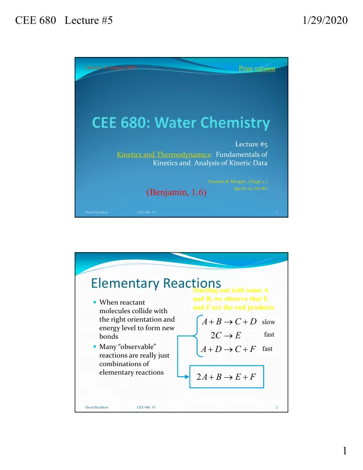
Elementary Reactions

 When reactant

molecules collide with the right orientation and energy level to form new bonds

 Many “observable”

reactions are really just combinations of elementary reactions

F E B A F C D A E C D C B A           2 2

David Reckhow CEE 680 #5 2

fast slow fast Starting out with some A and B, we observe that E and F are the end products

CEE 680 Lecture #5 1/29/2020 2

Cont.

 Elementary

reactions

 A single step in a

reaction sequence

 Involves 1 or 2 reactants and 1 or 2 products  Can be described by classical chemical

kinetics

David Reckhow CEE 680 #5 3

S&M: Fig. 2.11

• Pg. 72

Kinetics

 Examples

 Fe+2 oxidation by O2

 almost instantaneous at high pH  quite slow at low pH  high D.O. may help

 Oxidation of organic material  Formation of solid phases

 Aluminum hydroxide  Quartz sand

David Reckhow CEE 680 #5 4

CEE 680 Lecture #5 1/29/2020 3

Kinetics

 Base Hydrolysis of dichloromethane (DCM)

 Forms chloromethanol (CM) and chloride  Classic second order reaction (molecularity of 2)

 First order in each reactant, second order overall David Reckhow CEE 680 #5 5

dt Cl d dt CM d dt OH d dt DCM d OH DCM k Rate ] [ ] [ ] [ ] [ ] ][ [

  

      

Reaction Kinetics

 Irreversible reaction

 is one in which the reactant(s) proceed to product(s), but

there is no significant backward reaction,

 In generalized for, irreversible reactions can be represented

as:



aA + bB  Products

David Reckhow CEE 680 #5 6

i.e., the products do not recombine or change to form reactants in any appreciable amount. An example of an irreversible reaction is hydrogen and oxygen combining to form water in a combustion reaction. We do not observe water spontaneously separating into hydrogen and oxygen.

CEE 680 Lecture #5 1/29/2020 4

Reaction Kinetics: Reversibility

 A reversible reaction

 is one in which the reactant(s) proceed to product(s),

but the product(s) react at an appreciable rate to reform reactant(s).

 aA + bB  pP + qQ  Most reactions must be considered reversible

David Reckhow CEE 680 #5 7

An example of a reversible biological reaction is the formation of adenosine triphosphate (ATP) and adenosine diphosphate (ADP). All living organisms use ATP (or a similar compound) to store energy. As the ATP is used it is converted to ADP, the organism then uses food to reconvert the ADP to ATP.

Kinetic principles

 Law of Mass Action

 For elementary reactions

David Reckhow CEE 680 #5 8

where, CA = concentration of reactant species A, [moles/liter] CB = concentration of reactant species B, [moles/liter] a = stoichiometric coefficient of species A b = stoichiometric coefficient of species B k = rate constant, [units are dependent on a and b]

products bB aA

k

  

b B a AC

kC rate 

CEE 680 Lecture #5 1/29/2020 5

Reaction Kinetics (cont.)

 Reactions of order

“n” in reactant “c”

 When n=0, we have a

simple zero‐order reaction

David Reckhow CEE 680 #5 9

dc dt kcn  

dc dt k  

kt c c

• 



10 20 30 40 50 60 70 80 90 20 40 60 80 Concentration Time (min)

k mg l  10 / / min

Slope

Reaction Kinetics (cont.)

 When n=1, we

have a simple first‐order reaction

 This results in

an “exponential decay”

David Reckhow CEE 680 #5 10

dc dt kc  

1

c c e

• kt





10 20 30 40 50 60 70 80 90 20 40 60 80 Time (min) Concentration

k 



0 032

1

. min

CEE 680 Lecture #5 1/29/2020 6

Reaction Kinetics (cont.)

 This equation can

be linearized

 good for

assessment of “k” from data

David Reckhow CEE 680 #5 11

dc dt kc  

1 10 100 20 40 60 80 Time (min) Concentration (log scale)

kt c c

• 

 ln ln

k 



0 032

1

. min Slope

10 20 30 40 50 60 70 80 90 20 40 60 80 Time (min) Concentration

Reaction Kinetics (cont.)

 This results in

an especially wide range in rates

 More typical to

have 2nd order in each of two different reactants

David Reckhow CEE 680 #5 12

dc dt kc  

2

c c kc t

• 

 1 1

k L mg  0 0015 . / / min  When n=2, we have a simple second-order reaction

CEE 680 Lecture #5 1/29/2020 7

Reaction Kinetics (cont.)

 Again, the equation can be linearized

to estimate “k” from data

David Reckhow CEE 680 #5 13

dc dt kc  

2

0.02 0.04 0.06 0.08 0.1 0.12 20 40 60 80 Time (min) 1/Concentration

kt c c

• 

 1 1

k L mg  0 0015 . / / min

Slope

Comparison of Reaction Orders

 Curvature as order changes: 2nd>1st>zero

David Reckhow CEE 680 #5 14

10 20 30 40 50 60 70 80 90 20 40 60 80 Time (min) Concentration

Zero Order First Order Second Order

CEE 680 Lecture #5 1/29/2020 8

Reaction Kinetics (cont.)

 For most reactions, n=1 for each of two different

reactants, thus a second‐order overall reaction

David Reckhow CEE 680 #5 15

1 2 1 1c

kc dt dc  

1 1 5

min 10 9 . 3

  

 Lmg x k

 Many of these will have

• ne reactant in great

excess

 These become “pseudo‐ 1st order in the limiting reactant, as the reactant in excess really doesn’t change in concentration

2

c

1

c

10 20 30 40 50 60 70 80 90 20 40 60 80 Time (min) Concentration

Reaction Kinetics (cont.)

 Since C2 changes little

from its initial 820 mg/L, it is more interesting to focus on C1

 C1 exhibits simple 1st

• rder decay, called

pseudo‐1st order

 The pseudo‐1st order

rate constant is just the “observed rate” or kobs

David Reckhow CEE 680 #5 16

1 2 1 1c

kc dt dc  

t k

• bs

e c c





1 1

1 5 2

min 032 . ) 820 ( 10 9 . 3

 

   x kc kobs

CEE 680 Lecture #5 1/29/2020 9

Variable Kinetic Order

 Any reaction order, except n=1

David Reckhow CEE 680 #5 17

n

kc dt dc  

 

  



1 1 1

1 1 1

 

  

n n

• t

kc n c c

 kt

n c c

n

• n

1 1 1

1 1

  

 

Half‐lives

 Time required for initial concentration to drop to

half, i.e.., c=0.5co

 For a zero order reaction:  For a first order reaction:

David Reckhow CEE 680 #5 18

c c kt

• 



2 1

5 . kt c c

• 

 k c t

• 5

.

2 1 

c c e

• kt





2 1

5 .

kt

• e

c c





k k t 693 . ) 2 ln(

2 1

 

CEE 680 Lecture #5 1/29/2020 10

Kinetic problem

 If the half‐life of bromide in the presence of excess

chlorine is 13 seconds (pseudo‐1st order reaction,

 What is the pseudo‐1st order rate constant  how long does it take for 99% of the bromide to be

• xidized?

David Reckhow CEE 680 #5 19

HOCl Br HOBr Cl

k

    

 

Reactions in Series

David Reckhow CEE 680 #5 20

D C B A

k k k

     

3 2 1

• Fig. 2.9
• Pg. 68

k1=k2=k3=0.1 day-1

CEE 680 Lecture #5 1/29/2020 11

Reversible reaction kinetics

David Reckhow CEE 680 #5 21

For a general reversible reaction:

f b

k aA + bB pP + qQ k  And the rate law must consider both forward and reverse reactions:

A f A a B b b P p Q q

r = k C C - k C C

where, kf = forward rate constant, [units depend on a and b] kb = backward rate constant, [units depend on a and b] CP = concentration of product species P, [moles/liter] CQ = concentration of product species Q, [moles/liter] p = stoichiometric coefficient of species P q = stoichiometric coefficient of species Q

Reversible 1st order reactions

 Kinetic law  Eventually the

reaction slows and,

 Reactant

concentrations approach the equilibrium values

David Reckhow CEE 680 #5 22

• Fig. 2.10
• Pg. 69

] [ ] [

2 1

B k A k dt dB  

eq

K k k A B B k A k dt dB     

2 1 2 1

] [ ] [ ] [ ] [

CEE 680 Lecture #5 1/29/2020 12

Analysis of Rate Data

 Integral Method

 Least squares regression of linearized form

 Differential Method

 estimate instantaneous rate at known time and

reactant concentration

 Initial rate Method

 more rigorous, but slow

 Method of Excess

 only when 2 or more reactants are involved

David Reckhow CEE 680 #5 23

Kinetic model for equilibrium

D C B A D C B A

b f

k k

       

} }{ { B A k r

f f  David Reckhow CEE 680 #5 24

 Consider a reaction as

follows:

 Since all reactions are

reversible, we have two possibilities

 The rates are:  And at equilibrium the two

are equal, rf=rb

 We then define an

equilibrium constant (Keq)

} }{ { D C k r

b b 

A + B = C + D } }{ { } }{ { B A D C k k K

b f eq

  } }{ { } }{ { D C k B A k

b f



CEE 680 Lecture #5 1/29/2020 13

Kinetic model with moles

    B

A f f

B A k r   

David Reckhow CEE 680 #5 25

 In terms of molar concentrations, the rates are:  And at equilibrium the two are equal, rf=rb  And solving for the equilibrium constant (Keq)

    D

C b b

D C k r   

             

          

B A D C B A D C b f eq

B A D C B A D C k k K        

        D

C b B A f

D C k B A k     

To next lecture

David Reckhow CEE 680 #5 26