Effects of mis-specification of seasonal cointegrating ranks: An - PowerPoint PPT Presentation
Conference on Seasonality, Seasonal Adjustment and their implications for Short-Term Analysis and Forecasting 10-12 May 2006 Effects of mis-specification of seasonal cointegrating ranks: An empirical study Byeongchan Seong Sinsup Cho S. Y.
Conference on Seasonality, Seasonal Adjustment and their implications for Short-Term Analysis and Forecasting 10-12 May 2006 Effects of mis-specification of seasonal cointegrating ranks: An empirical study Byeongchan Seong Sinsup Cho S. Y. Hwang Sung K. Ahn
Effects of mis-specification of seasonal cointegrating ranks: An empirical study 1 Byeongchan Seong Pohang University of Science and Technology Sinsup Cho Seoul National University S. Y. Hwang Sookmyung Women’s University Sung K. Ahn Washington State University 1 Byeongchan Seong’s research was supported by the Post-doctoral Fellowship Program of Korea Science & Engineering Foundation (KOSEF). The research of Sinsup Cho, S. Y. Hwang, and Sung K. Ahn was supported by the Korea Research Foundation Grant (KRF- 2005-070-C00022) funded by the Korean Government (MOEHRD).
Co-integration (Engle & Granger, 1987) An m -dimensional I( d ) process y is co- t integrated, if there exists a vector β such that β ′ is an I( b ) process, b < y d , denoted by t CI( d , d-b ). Typically, processes are CI(1, 0), i.e., d =1 & b =0. The number of linearly independent vectors is called the co-integrating rank, denoted by r . “Disappearance” of the non-stationarity, or β ′ is attributable to the common y unit root in t feature (Engle & Kozicki, 1993), more specifically called, common trend in some or y . all of the elements of t
Seasonal Co-integration (Hylleberg, Engle, Granger & Yoo,1990) y with period s is A seasonal process t seasonally co-integrated at frequency f , if β ′ does not there exists a vector β such that y t θ i e corresponding have the seasonal unit root θ = π to the frequency f , f 2 . Since seasonal unit roots exist in conjugate pairs, there exists polynomial co-integrating ′ β + + β L β β L y vector such that ( ) does R I R I t e ± θ i not have the seasonal unit root
The characteristics of (seasonal) co- integration are concentrated in the error correction terms through the reduced ranks of the coefficient matrices. Φ − = + L L y C y ε * ( )( 1 ) − 1 t t t Φ − L L y * 4 ( )( 1 ) t = − + + + + C u C v C w C w ε − − − t t t t t 1 1 2 1 3 1 4 2 where = + + u L L y 2 ( 1 )( 1 ) , − − t t 1 1 = − + v L L y 2 , and ( 1 )( 1 ) − − t t 1 1 = − w L y 2 ( 1 ) − − t t 1 1 Statistical inference of co-integration involves reduced rank estimation in the error correction representation of the vector autoregressive model.
Multivariate Regression Model = + + + + z C x C x C x C x ε 1 1 2 2 3 3 4 4 Estimation: • Regression of on z x x x x , , , and 1 2 3 4 simultaneously. • Regression of on = z x j 1 K for each , , 4 j x if the ’s are uncorrelated. j • Partial regression of on z x adjusted for j k ≠ = x , j j 1 K for each , , 4 . k
Partial regression is especially useful if one C C of the ’s, say is of reduced rank. To j 1 C estimate with the reduced rank structure 1 imposed: • Regress z on x x x , , and and get the 2 3 4 r residual ; z • Regress x x x x on , , and and get the 1 2 3 4 r residual ; 1 • Reduded-rank regress on , r r z 1 as in Anderson (1951). In co-integration analysis Φ − = + L L y C y ε * ( )( 1 ) − 1 t t t • Regress ( − ( − L y L y 1 ) on lagged 1 ) and t t r get the residual ; y • Regress ( − y L y on on lagged 1 ) and − t t 1 r get the residual ; 1 • Reduced-rank regress r r on , y 1 as in Johansen (1988).
In seasonal co-integration analysis, more than C one ’s in j = + + + + z C x C x C θ x C θ x ε ( ) ( ) 1 1 2 2 3 3 4 4 C can be of reduced rank and some of the ’s j are dependent on the common parameter vector. C C C If and are of reduced rank and and 1 2 3 C depend on θ , then: 4 x x x Since the adjustment for , , and is 2 3 4 based on the full rank regression, partial reduced-rank regression of z on x is affected 1 C by over-specification of the rank of ; 2 x x x Since the adjustment for , , and is 1 2 3 based on the full rank regression, the C C dependence between and is ignored in 3 4 z x partial (reduced-rank) regression of on . 4
Seasonal Co-integration ′ ′ Φ − = + L L y α β u α R β v * 4 ( )( 1 ) − − t R R t R t 1 1 1 2 2 1 ′ ′ + + α β α β w ( ) − R I I R t 3 3 3 3 1 ′ ′ + − + + α β α β w ε ( ) − 2 R R I I t t 3 3 3 3 Lee (1992), Johansen & Schaumburg (1999), and Cubadda (2001) use partial reduced rank regression exploiting asymptotic zero correlations: • Lee assumes 3 = 3 = α β 0 and 0 ; I I • J&S uses the “switching” algorithm to α 3 β 3 α 3 , and β 3 ; estimate , , R R I I • Cubadda, in essence, estimates α 3 β 3 , , R R α 3 , and β 3 based on partial regression of I I − L y w 4 ( 1 ) on . − t t 1 These create over-specification problems.
Ahn & Reinsel (1994) and Ahn, Cho &Seong (2004) use an iterative scheme that incorporates • the co-integrating ranks at all the seasonal frequencies simultaneously and • the dependency among the coefficient matrices. But this requires the correct specification of the seasonal co-integrating ranks and is subject to over- and under-specification. (Furthermore, it can be computationally challenging.)
Simulation Study DGP (Ahn & Reinsel, 1994): ′ ′ − = + (1 L ) y α β u α β v 4 − − t t t 1 1 1 2 2 1 ′ ′ + + α β α β w ( ) − t 3 4 4 3 1 ′ ′ + − + + α β α β w ε ( ) − 2 t t 3 3 4 4 where ′ ′ = = α a a ( , ) ( 0 . 6 , 0 . 6 ) , 1 11 21 ′ ′ = = − α a a ( , ) ( 0 . 4 , 0 . 6 ) , 2 12 22 ′ ′ = = − α a a ( , ) ( 0 . 6 , 0 . 6 ) , 3 13 23 ′ ′ = = − α a a ( , ) ( 0 . 4 , 0 . 8 ) , 4 14 24 ′ ′ ′ ′ = = − = = β b β b ( 1 , ) ( 1 , 0 . 7 ) , ( 1 , ) ( 1 , 0 . 3 ) , 1 1 2 2 ′ ′ = = = = − β b β b ( 1 , ) ( 1 , 0 . 7 ) , ( 0 , ) ( 0 , 0 . 2 ) , 3 3 4 4
ρσ ⎛ ⎞ 1 = Ω = ⎜ ⎟ Cov ε ( ) t ρσ σ 2 ⎝ ⎠ 2 = ρ = − σ for 0 . 5 , 0 , 0 . 5 and 0 . 5 , 1 , 2 . Series length: 100 Replications: 1000 Nominal size: 0.05 Critical values from Johansen & Schaumburg (1999) and Lee & Siklos (1995) = > H r H r For : 0 vs : 0 for f f 0 1 = f H is rejected almost all the 0 , 1 / 2 , 1 / 4 , 0 cases regardless of under or over- specification. = > H r H r For : 1 vs : 1 , the results are f f 0 1 summarized below.
Table 1. Comparison of the rejection rates of 5% level tests for hypotheses in (6) for the = f frequency 1 / 2 . r r r C.I. ranks ( , , ) ρ σ 2 0 1 / 4 1 / 2 (0,0,1) (0,1,1) (0,2,1) (1,0,1) (1,1,1) (1,2,1) (2,0,1) (2,1,1) (2,2,1) 0.5 0.084 0.024 0.029 0.037 0.050 0.055 0.035 0.050 0.055 -0.5 1 0.084 0.037 0.043 0.039 0.058 0.059 0.040 0.059 0.059 2 0.081 0.062 0.070 0.035 0.060 0.061 0.034 0.059 0.061 0.5 0.086 0.026 0.029 0.035 0.056 0.059 0.040 0.057 0.062 0 1 0.083 0.035 0.038 0.040 0.060 0.065 0.042 0.060 0.065 2 0.088 0.053 0.056 0.041 0.064 0.066 0.040 0.063 0.066 0.5 0.082 0.020 0.025 0.045 0.056 0.058 0.051 0.055 0.057 0.5 1 0.075 0.025 0.033 0.040 0.060 0.065 0.044 0.060 0.063 2 0.079 0.043 0.047 0.043 0.064 0.063 0.046 0.063 0.063 • Significantly larger empirical sizes with under-specification for f =0 & 1/2. • Significantly smaller empirical sizes with under-specification for only one of f =0 & 1/2.
2 = ρ = σ Table 1-2. Means and mean squared errors for frequency 1/2 in case of 0 . 5 and 2 based on 1,000 replications. = − 22 = 2 = a a b CI ranks 0 . 4 0 . 6 0 . 3 12 r r r ( , , ) Mean MSE Mean MSE Mean MSE 0 1 / 4 1 / 2 (0,0,1) -0.3060 0.0182 0.7821 0.0624 0.2938 0.0002 (0,1,1) -0.2391 0.0541 0.6164 0.0566 0.2989 0.0004 (0,2,1) -0.2521 0.0462 0.6031 0.0534 0.2977 0.0009 (1,0,1) -0.3186 0.0148 0.6789 0.0196 0.2931 0.0002 (1,1,1) -0.3621 0.0107 0.5145 0.0443 0.3014 0.0000 (1,2,1) -0.3603 0.0102 0.5160 0.0430 0.3014 0.0001 (2,0,1) -0.3099 0.0148 0.6701 0.0181 0.2938 0.0001 (2,1,1) -0.3600 0.0108 0.5038 0.0463 0.3014 0.0001 (2,2,1) -0.3581 0.0104 0.5055 0.0449 0.3014 0.0001 • Serious biases occur with under- specification for the stationary parameters. • Biases are not serious with under- specification for the long-run parameter.
Recommend
More recommend
Explore More Topics
Stay informed with curated content and fresh updates.
