Effective Field Theory & New Physics @ LHC Sacha Davidson - PowerPoint PPT Presentation

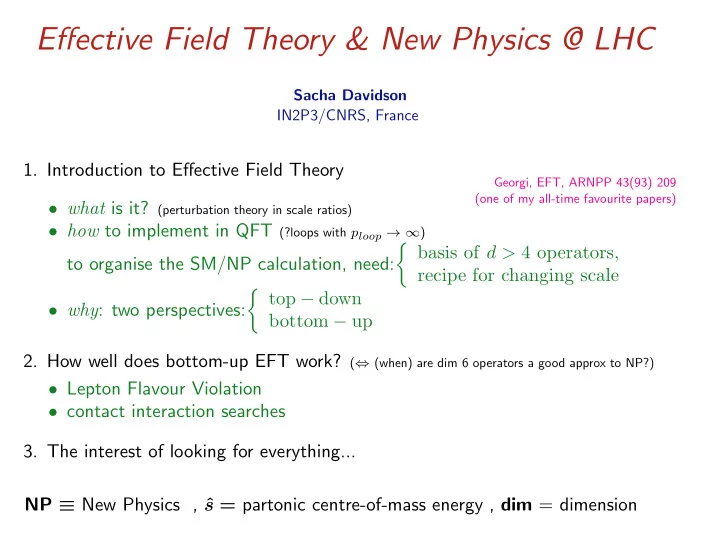
Effective Field Theory & New Physics @ LHC Sacha Davidson IN2P3/CNRS, France 1. Introduction to Effective Field Theory Georgi, EFT, ARNPP 43(93) 209 (one of my all-time favourite papers) • what is it? (perturbation theory in scale ratios) • how to implement in QFT (?loops with p loop → ∞ ) � basis of d > 4 operators , to organise the SM/NP calculation, need: recipe for changing scale � top − down • why : two perspectives: bottom − up 2. How well does bottom-up EFT work? ( ⇔ (when) are dim 6 operators a good approx to NP?) • Lepton Flavour Violation • contact interaction searches 3. The interest of looking for everything... NP ≡ New Physics , ˆ s = partonic centre-of-mass energy , dim = dimension

Georgi, EFT, ARNPP 43(93) 209 What is EFT? • there is interesting physics at all scales between “les deux infinis”

Georgi, EFT, ARNPP 43(93) 209 What is EFT? • there is interesting physics at all scales between “les deux infinis” • EFT = recipe to study observables at scale ℓ 1. choose appropriate variables to describe relevant dynamics ( eg use � E, � B and currents for radio waves, electrons and photons at LEP) � L ≫ ℓ → ∞ 2. 0th order interactions, by sending all parameters δ ≪ ℓ → 0 3. then perturb in ℓ/L and δ/ℓ

Georgi, EFT, ARNPP 43(93) 209 What is EFT? • there is interesting physics at all scales between “les deux infinis” • EFT = recipe to study observables at scale ℓ 1. choose appropriate variables to describe relevant dynamics ( eg use � E, � B and currents for radio waves, electrons and photons at LEP) � L ≫ ℓ → ∞ 2. 0th order interactions, by sending all parameters δ ≪ ℓ → 0 3. then perturb in ℓ/L and δ/ℓ Example : leptogenesis in the early Universe of age τ U ( τ U ∼ 10 − 24 sec) ⋆ processes with τ int ≫ τ U ...neglect! ⋆ processes with τ int ≪ τ U ...assume in thermal equilibrium! ⋆ processes with τ int ∼ τ U ...calculate this dynamics ⋆ can then do pert. theory in slow interactions and departures from thermal equil.

Pre -implementation of EFT in the SM , and for NP - take scale to be energy E : GeV → Λ NP ( > ∼ few TeV) (then do pert. theory in E/M, m/E for m ≪ E ≪ M ) - ...ummm...in QFT are loops, p loop → ∞ , p loop ≫ M ?

Pre -implementation of EFT in the SM , and for NP - take scale to be energy E : GeV → Λ NP ( > ∼ few TeV) (then do pert. theory in E/M, m/E for m ≪ E ≪ M ) - ...ummm...in QFT are loops, p loop → ∞ , p loop ≫ M ? � usually diverge on paper - theorists disturbed by loops: usually finite tiny effects in real world ⇒ machinery to regularise (loop integrals) and renormalise (coupling constants) - can extend regularisation/renormalisation to dim > 4 operators of EFT... ... but resulting EFT depends on details of how (eg put, or not, M ≫ E particles in loops?) ⋆ I use dim ensional reg ularisation ; restricts/defines the EFT I construct.

Pre -implementation of EFT in the SM , and for NP - take scale to be energy E : GeV → Λ NP ( > ∼ few TeV) (then do pert. theory in E/M, m/E for m ≪ E ≪ M ) - ...ummm...in QFT are loops, p loop → ∞ , p loop ≫ M ? � usually diverge on paper - theorists disturbed by loops: usually finite tiny effects in real world ⇒ machinery to regularise (loop integrals) and renormalise (coupling constants) - can extend regularisation/renormalisation to dim > 4 operators of EFT... ... but resulting EFT depends on details of how (eg put, or not, M ≫ E particles in loops?) ⋆ I use dim ensional reg ularisation ; restricts/defines the EFT I construct. ⇒ like in SM, EFT coupling constants (= operator coefficients) live in L rather than real world, are not observables... Can parametrise NP@LHC in S-matrix-based approach = “pseudo-observables”/(form factors), more general, less QFT-detail-dependent, more difficult?

EFT for the SM and heavy NP ( Λ NP ≫ m W ) 1. choose energy scale E of interest Λ NP > ∼ few TeV m W ∼ m h ∼ m t GeV ∼ m c , m b , m τ

EFT for the SM and heavy NP ( Λ NP ≫ m W ) 1. choose energy scale E of interest 2. include all particles with m < E Λ NP > ∼ few TeV f ′ , γ, g, Z, W, h, t m W ∼ m h ∼ m t f ′ , γ, g GeV ∼ m c , m b , m τ

EFT for the SM and heavy NP ( Λ NP ≫ m W ) 1. choose energy scale E of interest 2. include all particles with m < E 3. 0 th order theory (renormalisable interactions) :send → ∞ all M ≫ E Λ NP > ∼ few TeV f ′ , γ, g, Z, W, h, t L SM m W ∼ m h ∼ m t f ′ , γ, g L QED × QCD GeV ∼ m c , m b , m τ

EFT for the SM and heavy NP ( Λ NP ≫ m W ) 1. choose energy scale E of interest 2. include all particles with m < E 3. 0 th order theory (renormalisable interactions) :send → ∞ all M ≫ E 4. perturb in E/M (and m/E ) : allow d > 4 local operators ⇔ exchange of M ≫ E particles d counts field dims in interaction: ( ψψ )( ψψ ) ↔ dim 6 Λ NP > ∼ few TeV f ′ , γ, g, Z, W, h, t L SM + L (SM invar . operators) m W ∼ m h ∼ m t f ′ , γ, g L QED × QCD + L (QCD ∗ QED invar . ops) GeV ∼ m c , m b , m τ

To implement in practise, need operator basis + recipe to change scale at scale E , need a basis of operators, of dimension d > 4 1. E < m W : 3- and 4-point interactions of f ′ , γ, g ⇔ dimension 5,6,7 QCD*QED- invariant operators: Kuno-Okada CiriglianoKitanoOkadaTuscon γ µ µ g b +... µ µ µ g s e

µ g Parenthese: why 3,4-pt interactions? (not a “rule” to take dim 6?) +... g e eµ ) G A αβ G A (¯ αβ

µ g Parenthese: why 3,4-pt interactions? (not a “rule” to take dim 6?) +... g e bottom-up: for eg LFV, that is what is measurable . eµ ) G A αβ G A (¯ αβ want to run up starting from all data

µ g Parenthese: why 3,4-pt interactions? (not a “rule” to take dim 6?) +... g e bottom-up: for eg LFV, that is what is measurable . eµ ) G A αβ G A (¯ αβ want to run up starting from all data top-down: imagine an interaction ( eµ )( QQ ) for heavy quarks Q ∈ { c, b, t } contributes to µ → e conversion on a proton via: µ e µ e Q = ShifmanVainshteinZakarov C C eµ )( ¯ eµ ) G A αβ G A so below m Q , replace (¯ QQ ) → (¯ αβ Λ 2 Λ 2 NP m Q NP

To implement in practise, need operator basis + recipe to change scale at scale E , need a basis of operators, of dimension d > 4 1. E < m W : 3- and 4-point interactions of f ′ , γ, g ⇔ dimension 5,6,7 QCD*QED- invariant operators: γ µ µ g b +... µ µ µ g s e 2. E > m W : dim 6 SU (3) × SU (2) × U (1) -invar operators (neglect Majorana ν mass operators) Buchmuller-Wyler γ Z Gradkowski etal µ t +... µ µ µ µ e t

To implement in practise, need operator basis + recipe to change scale need a recipe to relate EFTs at different scales µ s t 1. when change EFTs ( eg at m W ): +... W match (= set equal) Greens functions µ b in both EFTs at the matching scale µ s ⇒ C V ( m W ) ∼ V ts 16 π 2 µ b G F C V (¯ sγb )(¯ µγµ )

To implement in practise, need operator basis + recipe to change scale need a recipe to relate EFTs at different scales µ s t 1. when change EFTs ( eg at m W ): +... W match (= set equal) Greens functions µ b in both EFTs at the matching scale µ s ⇒ C V ( m W ) ∼ V ts 16 π 2 µ b G F C V (¯ sγb )(¯ µγµ ) 2. Within an EFT: couplings (= operator coefficients) run and mix with scale. Can mix to other operators, (better?) constrained at other scales µ e γ τ τ e τ e γ s + ... ⇒ (¯ τστ )(¯ eσµ ) t µ µ τ τ 1) dominant part of 2-loop caln τ e e from (trivial 1-loop caln) 2 ! ⇒ t 2) sensitivity of µ → eγ to µ µ τ scalar ¯ ττ ¯ eµ operator ! (replace τ → t if you like)

Why do EFT: top-down vs bottom-up Two perspectives in EFT: top-down: EFT as the simple way to get the right answer know the high-scale theory = can calculate the coefficients of dim > 4 operators (because know cplings ⇔ other perturbative expansions) recall: EFT is perturbative expansion in scale ratios ( eg m B /m W ) useful as simple way to get answer to desired accuracy ( eg allows to resum QCD large logs)

Why do EFT: top-down vs bottom-up Two perspectives in EFT: top-down: EFT as the simple way to get the right answer know the high-scale theory = can calculate the coefficients of dim > 4 operators (because know cplings ⇔ other perturbative expansions) recall: EFT is perturbative expansion in scale ratios ( eg m B /m W ) useful as simple way to get answer to desired accuracy ( eg allows to resum QCD large logs) bottom-up: EFT as a parametrisation of ignorance not know NP masses, or couplings = other perturbative expansions ⇒ use lowest order EFT expansion (in scale ratio m SM / Λ NP ) to parametrise ... (?we hope??) many models ⇒ how well does bottom-up EFT work?

How well does bottom-up EFT work? (top-down: just do perturbative expansion to sufficient order...) 1. How precisely are the SM dynamics included? t / 16 π 2 ∼ y 2 (non-trivial problem: perturb in loops+ Yukawa+ gauge cplings y 2 c . In addition, matching at m W delicate due to appearance of Higgs vev which changes operator dimensions) 2. How good is lowest order EFT (dim 6 operators), as a parametrisation of New Physics?

First: what parameter space of dimension six operators can be probed? C s if > ǫ Suppose operator coefficient NP , detectable at scale ˆ Λ 2 s ˆ