EECS 70: Lecture 27. Recap Joint distribution. Joint and - - PowerPoint PPT Presentation

EECS 70: Lecture 27.

Joint and Conditional Distributions.

• 1. Recap of variance of a random variable
• 2. Joint distributions
• 3. Recap of indep. rand. variables: Variance of B(n,p)
• 4. Conditioning of Random Variables (revisit G(p))

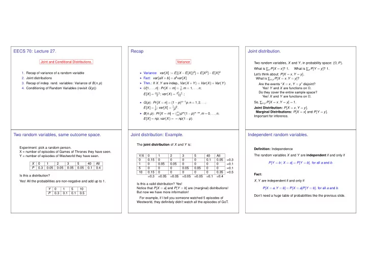
Recap

Variance

◮ Variance: var[X] := E[(X −E[X])2] = E[X 2]−E[X]2 ◮ Fact: var[aX +b] = a2var[X] ◮ Thm.: If X,Y are indep., Var(X +Y) = Var(X)+Var(Y). ◮ U[1,...,n] : Pr[X = m] = 1 n,m = 1,...,n;

E[X] = n+1

2 ; var(X) = n2−1 12 .; ◮ G(p) : Pr[X = n] = (1−p)n−1p,n = 1,2,...;

E[X] = 1

p; var[X] = 1−p p2 . ◮ B(n,p) : Pr[X = m] =

n

m

• pm(1−p)n−m,m = 0,...,n;

E[X] = np; var(X) = = np(1−p).

Joint distribution.

Two random variables, X and Y, in probability space: (Ω,P). What is ∑x P[X = x]? 1. What is ∑y P[Y = y]? 1. Let’s think about: P[X = x,Y = y]. What is ∑x,y P[X = x,Y = y]? Are the events “X = x, Y = y” disjoint? Yes! Y and X are functions on Ω. Do they cover the entire sample space? Yes! X and Y are functions on Ω. So, ∑x,y P[X = x,Y = y] = 1. Joint Distribution: P[X = x,Y = y]. Marginal Distributions: P[X = x] and P[Y = y]. Important for inference.

Two random variables, same outcome space.

Experiment: pick a random person. X = number of episodes of Games of Thrones they have seen. Y = number of episodes of Westworld they have seen. X 1 2 3 5 40 All P 0.3 0.05 0.05 0.05 0.05 0.1 0.4 Is this a distribution? Yes! All the probabilities are non-negative and add up to 1. Y 1 5 10 P 0.3 0.1 0.1 0.5

Joint distribution: Example.

The joint distribution of X and Y is: Y/X 1 2 3 5 40 All 0.15 0.1 0.05 =0.3 1 0.05 0.05 =0.1 5 0.05 0.05 =0.1 10 0.15 0.35 =0.5 =0.3 =0.05 =0.05 =0.05 =0.05 =0.1 =0.4 Is this a valid distribution? Yes! Notice that P[X = a] and P[Y = b] are (marginal) distributions! But now we have more information! For example, if I tell you someone watched 5 episodes of Westworld, they definitely didn’t watch all the episodes of GoT.

Independent random variables.

Definition: Independence The random variables X and Y are independent if and only if P[Y = b | X = a] = P[Y = b], for all a and b. Fact: X,Y are independent if and only if P[X = a,Y = b] = P[X = a]P[Y = b], for all a and b. Don’t need a huge table of probabilities like the previous slide.

Independence: examples.

Example 1 Roll two dices. X,Y = number of pips on the two dice. X,Y are independent. Indeed: P[X = a,Y = b] = 1/36,P[X = a] = P[Y = b] = 1/6. Example 2 Roll two dices. X = total number of pips, Y = number of pips on die 1 minus number on die 2. X and Y are not independent. Indeed: P[X = 12,Y = 1] = 0 = P[X = 12]P[Y = 1] > 0.

Mean of product of independent RVs.

Theorem Let X,Y be independent RVs. Then E[XY] = E[X]E[Y]. Proof:

Recall that E[g(X,Y)] = ∑x,y g(x,y)P[X = x,Y = y]. Hence, E[XY] = ∑

x,y

xyP[X = x,Y = y] = ∑

x,y

xyP[X = x]P[Y = y], by ind. = ∑

x

• ∑

y

xyP[X = x]P[Y = y]

• = ∑

x

• xP[X = x]
• ∑

y

yP[Y = y]

• = ∑

x

xP[X = x]E[Y] = E[X]E[Y].

Variance of sum of two independent random variables

Theorem: If X and Y are independent, then Var(X +Y) = Var(X)+Var(Y). Proof: Since shifting the random variables does not change their variance, let us subtract their means. That is, we assume that E(X) = 0 and E(Y) = 0. Then, by independence, E(XY) = E(X)E(Y) = 0. Hence, var(X +Y) = E((X +Y)2) = E(X 2 +2XY +Y 2) = E(X 2)+2E(XY)+E(Y 2) = E(X 2)+E(Y 2) = var(X)+var(Y).

Examples.

(1) Assume that X,Y,Z are (pairwise) independent, with E[X] = E[Y] = E[Z] = 0 and E[X 2] = E[Y 2] = E[Z 2] = 1. Then E[(X +2Y +3Z)2] = E[X 2 +4Y 2 +9Z 2 +4XY +12YZ +6XZ] = 1+4+9+4×0+12×0+6×0 = 14. (2) Let X,Y be independent and U{1,2,...,n}. Then E[(X −Y)2] = E[X 2 +Y 2 −2XY] = 2E[X 2]−2E[X]2 = 1+3n +2n2 3 − (n +1)2 2 .

Variance: binomial.

E[X 2] =

n

∑

i=0

i2 n i

• pi(1−p)n−i.

= Really???!!##... Too hard! Ok.. fine. Let’s do something else. Maybe not much easier...but there is a payoff.

Variance of Binomial Distribution.

Flip coin with heads probability p. X- how many heads? Xi = 1 if ith flip is heads

• therwise

E(X 2

i ) = 12 ×p +02 ×(1−p) = p.

Var(Xi) = p −(E(X))2 = p −p2 = p(1−p). p = 0 = ⇒ Var(Xi) = 0 p = 1 = ⇒ Var(Xi) = 0 X = X1 +X2 +...Xn. Xi and Xj are independent: Pr[Xi = 1|Xj = 1] = Pr[Xi = 1]. Var(X) = Var(X1 +···Xn) = np(1−p).

Conditioning of RVs

Recall conditioning on an event A P[X = k | A] = P[(X = k)∩A] P[A] Conditioning on another RV P[X = k | Y = m] = P[X = k,Y = m] P[Y = m] = pX|Y(x | y) pX|Y(x | y) is called the conditional distribution or conditional probability mass function (pmf) of X given Y pX|Y(x | y) = pXY(x,y) pY(y)

Conditional distributions

X | Y is a RV:

∑

x

pX|Y(x | y) = ∑

x

pXY(x,y) pY(y) = 1 Multiplication or Product Rule: pXY(x,y) = pX(x)pY|X(y | x) = pY(y)pX|Y(x | y) Total Probability Theorem: If A1, A2, ..., AN partition Ω, and P[Ai] > 0 ∀i, then pX(x) =

N

∑

i=1

P[Ai]P[X = x | Ai] Nothing special about just two random variables, naturally extends to more. Let’s visit the mean and variance of the geometric distribution using conditional expectation.

Revisiting mean of geometric RV X ∼ G(p)

X is memoryless P[X = n +m | X > n] = P[X = m]. Thus E[X | X > 1] = 1+E[X]. Why? (Recall E[g(X)] = ∑l g(l)P[X = l]) E[X | X > 1] =

∞

∑

k=1

kP[X = k | X > 1] =

∞

∑

k=2

kP[X = k−1] (memoryless) =

∞

∑

l=1

(l +1)P[X = l] (l = k −1) = E[X +1] = 1+E[X]

Revisiting mean of geometric RV X ∼ G(p)

X is memoryless P[X = k +m | X > k] = P[X = m]. Thus E[X | X > 1] = 1+E[X]. We have E[X] = P[X = 1]E[X | X = 1]+P[X > 1]E[X | X > 1]. ⇒ E[X]= p.1+(1−p)(E[X]+1) ⇒ E[X] = p +1−p +E[X]−pE[X] ⇒ pE[X] = 1 ⇒ E[X] = 1 p Derive the variance for X ∼ G(p) by finding E[X 2] using conditioning.

Summary of Conditional distribution

For Random Variables X and Y, P[X = x | Y = k] is the conditional distribution of X given Y = k P[X = x | Y = k] = P[X = x,Y = k] P[Y = k] Numerator: Joint distribution of (X,Y). Denominator: Marginal distribution of Y. (Aside: surprising result using conditioning of RVs): Theorem: If X ∼ Poisson(λ1), Y ∼ Poisson(λ2) are independent, then X +Y ∼ Poisson(λ1 +λ2). “Sum of independent Poissons is Poisson.”

Summary.

Joint and Conditional Distributions. Joint distributions:

◮ Normalization: ∑x,y P[X = x,Y = y] = 1. ◮ Marginalization: ∑y P[X = x,Y = y] = P[X = x]. ◮ Independence: P[X = x,Y = y] = P[X = x]P[Y = y] for all

x,y. E[XY] = E[X]E[Y]. Conditional distributions:

◮ Sum of independent Poissons is Poisson. ◮ Conditional expectation: useful for mean & variance

calculations