EE 6882 Statistical Methods for Video Indexing and Analysis Fall - - PDF document

SLIDE 1

1

1

EE 6882 Statistical Methods for Video Indexing and Analysis

Fall 2004

• Prof. Shih-Fu Chang

http://www.ee.columbia.edu/~sfchang Lecture 2 Part B (9/15/04)

2 EE6882-Chang

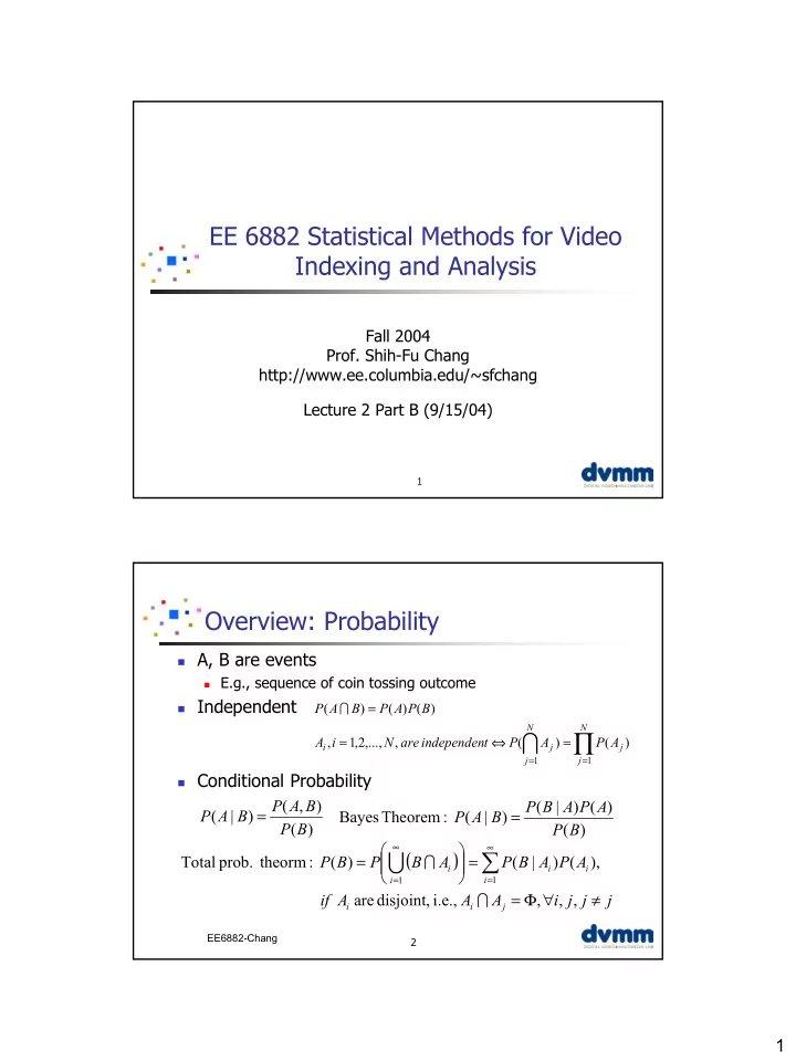
Overview: Probability

A, B are events

E.g., sequence of coin tossing outcome

Independent Conditional Probability

∏

= =

= ⇔ = =

N j j N j j i

A P A P t independen are N i A B P A P B A P

1 1

) ( ) ( , ,..., 2 , 1 , ) ( ) ( ) (

∩

∩

) ( ) , ( ) | ( B P B A P B A P = ) ( ) ( ) | ( ) | ( : Theorem Bayes B P A P A B P B A P =

( )

j j j i A A A if A P A B P A B P B P

j i i i i i i i

≠ ∀ Φ = =         =

∑

∞ = ∞ =

, , , i.e., disjoint, are , ) ( ) | ( ) ( : theorm prob. Total

1 1

∩ ∩

∪

SLIDE 2

2

3 EE6882-Chang

Probability

Independence & mutual exclusion (uncorrelated) different

t independen Not B P A P B A P ) ( ) ( ) ( But ⇒ ≠ ∩

B A

ed uncorrelat B P A P B A P ) ( ), ( , ) ( ⇒ ≠ = ∩

Probability of random variable

Cumulative distribution function (cdf) Probability density function (pdf)

( ] { }

x ,

• X

Prob x FX ∞ ∈ = ) (

{ }

x x X X

x d x dF x P

= ′

′ ′ = = = ) ( x X Prob ) (

, , i , ) x x ( ) x ;...; x P( iff t independen are ,...,

k 1 k i n 1 1

k 1

N n P x x x x

n k i i N

n

≤ ≤ = ≤ ≤

∏

=

4 EE6882-Chang

Probability

Joint distribution Joint density Marginal distribution Conditional probability

{ }

y Y x, X Prob y x F

Y X

≤ ≤ = ) , (

, y y x x Y X Y X

y x F y x y x f

= ′ = ′

′ ′ ′ ∂ ′ ∂ ∂ =

, , 2 ,

) , ( ) , (

∫

=

R Y X X

dy y x f x f ) , ( ) (

,

dy y f y x f x y f x f x y f y x f Bayes

Y X Y X Y X

) ( ) | ( ) ( f : theorem prob. Total ) ( ) ( ) ( ) ( : theorem

X

∫

= =

y & both x

• f

function a : note , ) ( ) , ( ) (

,

y f y x f y x f

Y Y X X

=

SLIDE 3

3

5 EE6882-Chang

Probability

Expectation (expected value)

E.g., mean, variance, moments, central moments Integral become summation if x is discrete

∫ ∫

= = dx x f x g x g E dx x xf x E

X X

) ( ) ( )) ( ( , ) ( ) (

6 EE6882-Chang

Entropy

• Entropy (bits)
• Given same mean and variance,
• Gaussian has the max entropy
• Dirac delta distribution has the

lowest entropy,

• For discrete x and arbitrary function

f(.)

• Processing never increases entropy

for discrete variables

• Because prob. cannot be split to two

different values after processing

∑

=

− =

m i i i

p p H

1 2

log

dx x p x p H ) ( log ) (

2

∫

∞ ∞ −

− =

) 2 ( log 5 .

2

σ π + =

gau

H

a x if a x if a x = ∞ ≠ = − ) ( δ

−∞ = ⇒

d

H ) ( )) ( ( x H x f H ≤

SLIDE 4

4

7 EE6882-Chang

Relative Entropy

Also called Kullback-Leibler (K-L) Distance

A measure of ‘distance’ between 2 distributions

• Not necessarily symmetric, may not satisfy triangular

inequality

( )

dx x p x q x q

• r

x p x q x q x q x p D

• x

KL

∫ ∑

∞ ∞

= = ) ( ) ( log ) ( ) ( ) ( log ) ( ) ( ), (

( ) ( )

⋅ = ⋅ = ≥ q p ff i and DKL ,

8 EE6882-Chang

Mutual Information

• Reduction in uncertainty about one variable due to the knowledge
• f the other one, e.g., p(x) and q(y). Can be different variables

and different distributions.

• I(p;q)=0 iff p, q are independent
• Symmetric I(p;q)= I(q;p)
• But I(p;q) is not a metric

E.g., if p(x)=q(y), I(p;q) may not be 0

H(p, q) = H(p) + H(q|p) = H(q) + H(p|q)

( )

) ( ) ( ), , ( prob. joint the is where , ) ( ) ( ) , ( log ) , ( ) | ( ) ( ) ; (

x y

y q x p y x r D r(x,y) y q x p y x r y x r q p H p H q p I

KL

= = − =

∑∑

;

H(p,q) H(p|q) H(q|p) H(p) H(q) I(p,q)

SLIDE 5

5

9 EE6882-Chang

Random Number Generation

T u v P(u) u P(v) v What’s the relationship between u & v? F(u) u F(v) v 1 u’ 1 v’ t t

( ) ( ) ( )

u F F v u F v F

U V U V

′ = ′ ′ = ′

−1

• Note all random number generators in Matlab use rand() or randn() (I.e.,

‘uniform’ or ‘normal’ distribution)

• Remember to change the initial state of rand() & randn()
• E,g: ini-sta; rand(‘state’,ini-sta); randn(‘state’, ini-sta);
• If there is no analytical form for CDF, how to generate samples?

hist equal demo

10 EE6882-Chang

Gaussian Distribution

• Gaussian distribution
• Multivariate Gaussian

/ to from distance s Mahalanobi 997 . ] 3 Pr[ 95 . ] 2 Pr[ 68 . ] Pr[ σ µ µ σ µ σ µ σ µ − = ≅ ≤ − ≅ ≤ − ≅ ≤ − x r x x x x

( ) 

     − −

=

2 2

2 1 2

2 1 ) (

µ σ

πσ

x

e x p

( )

( ) ( )

matrix : vectors l dimensiona

• D

are , 2 1 ) (

1

2 1 2 /

D D where e p

T

D

× =

      − − −

−

Σ µ x Σ x

µ x Σ µ x

π

x2 x1

General Σ

x2 x1

        =

2 2 2 1

σ σ Σ

SLIDE 6

6

11 EE6882-Chang

Generate Samples Of Gaussian

function) (error 2 ) ( , 2 1 2 1 2 1 ) ( ) ( 2 1 ) ( 1 , ), 1 , | ( ~

2 1 2

2 2

∫ ∫

− ∞ − −

= +       = = = → = =

x t x x

dt e x erf where x erf dt t p x F e x p x N x π π σ µ

Step 1: Generate uniform samples

u F uniform u

u =

), 1 , ( ~

Step 2:

( ) ( ) ( )

) 1 2 ( 2 1 2 1 2 1

1

− = = → +       = = =

−

u erfinv u F x x erf x F u u F

X X U

Step 3: Generate

2

2 1 1 : 1

2 1 ) ( ) , | ( ~

d

x D d D D

e x p I x N x

− =

Π = π

Step 4: Scale & shift

( )

Σ + Σ = , ~

2 / 1

µ µ N x z

See GauNorm demo 12 EE6882-Chang

Random Generators In Matlab

Generate normally distributed samples. 1-D Other similar generators include Betarnd, binornd, chi2rnd, exprnd, evrnd, frnd, gamrnd, geornd, hygernd, iwishrnd, lognrnd, nbinrnd, ncfrnd, nctrnd, ncx2rnd, normrnd, poissrnd, raylrnd, trnd, unidrnd, unifrnd, wblrnd, wblrnd, wishrnd normrnd Generate multivariate normally distributed samples. A similar generator is mvtrnd, which creates multivariate t distribution. mvnrnd A function to generate samples with specified distribution, 1-D random Create samples with standard normal distribution, N(0, 1), 1-D randn Generate uniformly distributed samples in the interval [0,1], 1-D rand Purpose Function Name

NOTE: All of these generators, except rand and randn, are included in Statistical Toolbox.

See ‘randtool’ and ‘disttool’ demos in Matlab

SLIDE 7

7

13 EE6882-Chang

Gaussian Used In Regression

                          −               Σ Σ Σ Σ                 −         − Σ = −

− y x yy xy yx xx T y x D

y x y x y x p D µ µ µ µ π

1 2 /

2 1 exp ) 2 ( 1 ) , ( Gaussian 2

( )

xy xx yx yy x xx yx y

x y N x y p Σ Σ Σ − Σ − Σ Σ + =

− − 1 1

), ( ) | ( µ µ

Model the joint distribution Conditional distribution of y given x

x p(y|x)

14 EE6882-Chang

Discriminant Analysis

• discriminant function: closeness

. . . . . . . . . x x x

x(1) x(2)

xx x

C1 C2

Given a feature vector Discriminant functions Assign to class if

x

• ( ),

1,2

k

g x k =

• x
• k

( ) ( ),

k i

g x g x i k > ≠

• (

)

:

k k k

g =1/distance x,C where C centroid of class k

• ( |

)

k k

g prob x C =

• x

Likelihood P(x|C1) P(x|C2)

2 1 1 1 1 2

( | ) ( , ) (1 ) p x C N

• r Gaussian Mixture

N N µ σ α α = + −

• discriminant function: Likelihood

SLIDE 8

8

15 EE6882-Chang

Discriminant Analysis

Example of discriminant function

Linear and quadratic discriminant

1 2

( ) g x ax bx = +

• 1

2

2 2 1 2

( ) g x ax bx cx x = + +

• +

+ + +

• +

x(1) x(2) Decision boundary

+ + + + + + + + +

• o
• +

+

( ) g x >

• ( )

g x <

• +

+ + +

• +

x(1) x(2) Decision boundary

• +

+ + + + + + +

16 EE6882-Chang

Decision Tree: Non-parametric

x(1) x(2)

• +

+

x(3)

+ +

• o
• +

+ + + + + + + +

TH1 TH2 x(2)>TH1 C+ x(1)>TH2 Co Y N Y N C+

Find most opportunistic

dimension in each step

Selection criterion

Entropy Variance before / after

Stop criterion

Avoid overfitting

See ‘classification’ demo in statistics toolbox

SLIDE 9

9

17 EE6882-Chang

Clustering

Training data Unsupervised learning K-mean clustering

Fix K values Initialize the representative of each cluster Map samples to closest cluster Re-compute the centers

{ } { }

( )

i

x label i ? +

x(1) x(2)

• +

+ + + +

• +

+ ++ +

…

• C1

C2 C3 CK

1 2

, ,..., , , ) , ), '

N i k i k i k'

x x x samples for i=1,2,...,N, x C if Dist(x C Dist(x C k k end → < ≠

18 EE6882-Chang

Gaussian Used In Classification

( ) ( ) ( )

• evidence

prior j likelihood j j

x p w p w x p x when x p x if w x ) ( ) ( ) | ( w p classifier MAP j i , w w p ,

j i j

• =

≠ ≥ →

( )

Gaussians by modeled be can ) | ( ) | ( max arg w p uniform : tion classifica ML

j

w x p w x p w if

w j =

⇒

SLIDE 10

10

19 EE6882-Chang

Mixture Of Gaussians

• Given data x1, …, xN , define log-likelihood:
• Define zn as a random variable, indicating

the component generating the sample

( )

( ) ( )

∑ ∑ ∑ ∑

= − Σ − −

−

Σ = Σ = = =

Z z x x z D z z z z z z z

z z T z

e x N z x p z p z x p x p

1 2 1 2 /

1

) 2 ( 1 , ) | ( ) ( ) , ( ) (

µ µ

π π µ π

x p(x) π0 π1

( )

∑

=

Σ + Σ =

N n n n

x N x N l

1 1 1 1

) , ( ) , ( log µ π µ π

( )

} , , , { , , 1

1 1 component

• f

Σ Σ = = = =

     

µ µ θ θ τ x z p posteriers

i i i ity responsibl

• Real distributions seldom follow a single Gaussian mixture of

Gaussians

20 EE6882-Chang

Expectation-Maximization (EM)

EM for estimating θ and

.

Follow ‘divide and conquer’ principle In iteration step t:

( ) ( ) ( )

( )

( ) ( )

( )

∑

Σ Σ =

j t j t j n i t i t i n i t i n

x N x N n Expectatio , | , | : µ π µ π τ

( ) ( ) ( )

∑ ∑

=

+ n t i n n n t i n 1 t i

x Maximation τ τ µ :

( ) ( ) ( )

( )

( )

( )

( )

∑ ∑

+ + +

− − = Σ

n t i n n T 1 t i n 1 t i n t i n 1 t i

x x τ µ µ τ Weight from component i Divide data to each group, Compute mean and variance from each group

i

τ

SLIDE 11

11

21 EE6882-Chang

Maximum Likelihood Through EM

• Maximization of l(θ) directly is hard due to log_of_sum
• Instead, look at
• Jensen’s Inequality

( )

∑ ∑

=

=

N n z n z

x p l

1

| , log ) ( θ θ

θ θ θ θ θ

• f

estimation : ), ( ) ( ) ( current l l l

t t

− = ∆ ( )

∑ ∑

=

=

N n z t n t

z x p l

1

| , log ) ( θ θ

{ } ( ) { } ( ) ( ) { } ( ) ( ) { } ( ) ( ) ( ) { } ( ) { } ( )

x f E x E f convex, is f If p where x p x p x x f g e x g f E x g E f x f E x E f concave, is f If

i i i i i i i i

≤ = ≥         = ≥ ≥

∑ ∑ ∑

1 , log log ) log( ., . Total log likelihood

22 EE6882-Chang

Maximum Likelihood Through EM (2)

• Derivation based on Jensen’s Inequality,
• Now estimate θt+1 by maximizing Q
• So in the expectation step, compute , the ‘responsibility ‘ of

component z for sample xn

• In the maximization step, take derivative of Q to θ, and find the

new estimate for θ

( )

( ) ( ) ( )

) | ( | , | , log , | ) (

1 ) ( ) ( t t n n N n z t n l l

Q z x p z x p x z p l

t

θ θ θ θ θ θ

θ θ

= ≥ ∆

∑∑

= − =

) | ( max arg

1 t t

Q θ θ θ

θ

=

+

( ) ( )

const z x p x z p Q

n N n z ectation t n t

t

+ =∑∑

=

• hidden

&

• bserved
• f

likelihood joint 1 current with z

• ver

exp

| , log , | ) | ( θ θ θ θ

θ z n

τ

“Auxiliary function”

SLIDE 12

12

23 EE6882-Chang

EM Always Improves Likelihood

) ( ) | ( ) | ( max ) | ( , ) | ( ) | ( ) ( ) ( ) (

1 1 1 1 1

≥ ∆ ∴ = ≥ = = ≥ − = ∆

+ + + + + t t t t t t t t t t t t t

l Q Q Q Q Note Q l l l θ θ θ θ θ θ θ θ θ θ θ θ θ θ

θ

( ) ( )

const z x p x z p Q

n N n z ectation t n t

t

+ = ∑∑

=

• hidden

&

• bserved
• f

likelihood joint 1 current with z

• ver

exp

| , log , | ) | ( θ θ θ θ

θ

• Why does EM always improve l(θ) ?
• General steps of EM:
• Define likelihood model with parameters θ
• Identify hidden variables z
• Derive the auxiliary function and the E and M equations
• In each iteration, estimate the posteriors of hidden variables
• Re-estimate the model parameters. Repeat until stop

24 EE6882-Chang

Paper List for Fall 2004

Updated paper list available at the course web site Topics

Content-based image search Web image search Media fingerprinting Image classification

Bayesian, Boosting, SVM Relevance feedback

Document clustering HMM and video classification Language models and applications in multimedia IR

Feel free to propose topics