ECO 317 Economics of Uncertainty Fall Term 2009 Notes for Lectures - PDF document

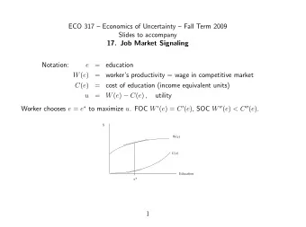
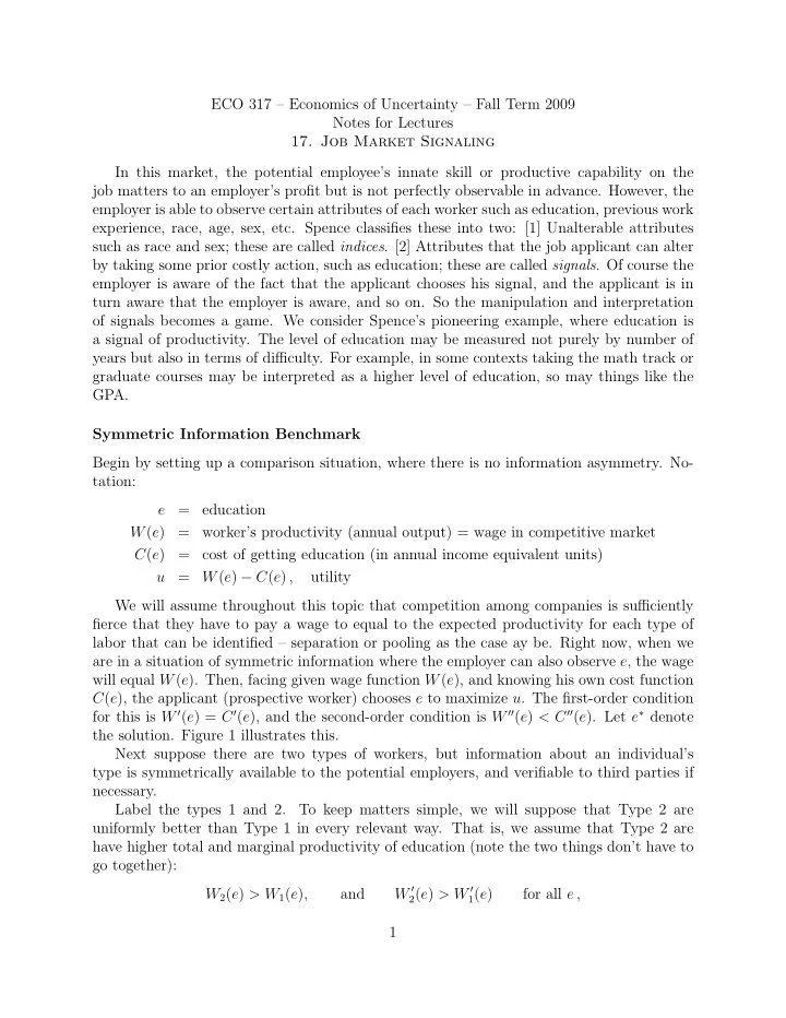
ECO 317 – Economics of Uncertainty – Fall Term 2009 Notes for Lectures 17. Job Market Signaling In this market, the potential employee’s innate skill or productive capability on the job matters to an employer’s profit but is not perfectly observable in advance. However, the employer is able to observe certain attributes of each worker such as education, previous work experience, race, age, sex, etc. Spence classifies these into two: [1] Unalterable attributes such as race and sex; these are called indices . [2] Attributes that the job applicant can alter by taking some prior costly action, such as education; these are called signals . Of course the employer is aware of the fact that the applicant chooses his signal, and the applicant is in turn aware that the employer is aware, and so on. So the manipulation and interpretation of signals becomes a game. We consider Spence’s pioneering example, where education is a signal of productivity. The level of education may be measured not purely by number of years but also in terms of difficulty. For example, in some contexts taking the math track or graduate courses may be interpreted as a higher level of education, so may things like the GPA. Symmetric Information Benchmark Begin by setting up a comparison situation, where there is no information asymmetry. No- tation: e = education W ( e ) = worker’s productivity (annual output) = wage in competitive market C ( e ) = cost of getting education (in annual income equivalent units) = W ( e ) − C ( e ) , utility u We will assume throughout this topic that competition among companies is sufficiently fierce that they have to pay a wage to equal to the expected productivity for each type of labor that can be identified – separation or pooling as the case ay be. Right now, when we are in a situation of symmetric information where the employer can also observe e , the wage will equal W ( e ). Then, facing given wage function W ( e ), and knowing his own cost function C ( e ), the applicant (prospective worker) chooses e to maximize u . The first-order condition for this is W ′ ( e ) = C ′ ( e ), and the second-order condition is W ′′ ( e ) < C ′′ ( e ). Let e ∗ denote the solution. Figure 1 illustrates this. Next suppose there are two types of workers, but information about an individual’s type is symmetrically available to the potential employers, and verifiable to third parties if necessary. Label the types 1 and 2. To keep matters simple, we will suppose that Type 2 are uniformly better than Type 1 in every relevant way. That is, we assume that Type 2 are have higher total and marginal productivity of education (note the two things don’t have to go together): W ′ 2 ( e ) > W ′ W 2 ( e ) > W 1 ( e ) , and 1 ( e ) for all e , 1

$ W(e) C(e) Education e* Figure 1: Complete Information – One Type of Worker and that Type 2 have lower total and marginal cost of getting educated: C ′ 2 ( e ) < C ′ C 2 ( e ) < C 1 ( e ) , and 1 ( e ) for all e . The comparison of the net marginal benefits of education across the types, namely W ′ 2 ( e ) − C ′ 2 ( e ) > W ′ 1 ( e ) − C ′ 1 ( e ) for all e , constitutes the Mirrlees-Spence “single-crossing property” in this context. Under symmetric information, each type chooses its optimal level of education. And the assumptions we have made ensure that e ∗ 2 > e ∗ 1 . Figure 2 illustrates this. $ W (e) 2 R L W (e) 1 K C (e) C (e) 1 2 Q J P H Education * * e e 1 2 Figure 2: Complete Information – Two Types of Workers 2

Asymmetric Information Continue with the two types above, but now suppose each applicant’s type is private in- formation. Suppose an employer tries to achieve the complete information outcome above, using the applicant’s verifiable education choices as an indication of their type. That is, the employer offers a wage contingent on the education level: “If you have education level e ∗ 2 , you will be paid W 2 ( e ∗ 2 ); if you have education level e ∗ 1 , you will be paid W 1 ( e ∗ 1 ).” Now someone who is truly Type 1, by getting education e ∗ 2 , can get paid more. Is this worthwhile given Type 1’s higher cost of getting that extra education? Yes, if W 2 ( e ∗ 2 ) − C 1 ( e ∗ 2 ) > W 1 ( e ∗ 1 ) − C 1 ( e ∗ 1 ) . In Figure 2, this is the comparison of the heights QR and JK. In the figure the two are shown almost equal; this is deliberately done, to show and remind you that in general the comparison could go either way. It is thus possible that Type 1 will mimic the actions of Type 2 to be accepted as that type and paid a higher wage. But if this goes on, the employers will be paying W 2 ( e ∗ 2 ) to several people whose true productivity is only W 1 ( e ∗ 2 ). This will result in losses; therefore such contracts cannot prevail in equilibrium. Note that the converse is not true: Type 2 does not want to mimic Type 1’s choice, because W 2 ( e ∗ 2 ) − C 2 ( e ∗ 2 ) > W 2 ( e ∗ 1 ) − C 2 ( e ∗ 1 ) > W 1 ( e ∗ 1 ) − C 2 ( e ∗ 1 ) , where the first inequality follows from the fact that e ∗ 2 is optimal for Type 2, and the second because W 2 ( e ) > W 1 ( e ) for all e . In Figure 2, these inequalities correspond to PR > HL and HL > HK respectively. To overcome Type 1’s temptation to mimic Type 2 and achieve separation of types, the level of education needed as evidence of a person being Type 2 must be higher. Try a contract of the form: There is a threshold level of education E such that workers with education e ≥ E will be regarded as Type 2 and paid W 2 ( e ), workers with education e < E will be regarded as Type 1 and paid W 1 ( e ). To ensure that Type 1 does not want to mimic Type 2, we need W 1 ( e ∗ 1 ) − C 1 ( e ∗ 1 ) ≥ W 2 ( E ) − C 1 ( E ) . (The use of the weak inequality ≥ , not the strict > , incorporates an indifference-breaking assumption in favor of one’s true type; it is harmless since one can always get an outcome arbitrarily close to this by changing E to an infinitesimally higher level.) In Figure 3, the 2 (min), where JK = J ′ K ′ . smallest value of E compatible with this condition is e s For the case of interest here, Type 1 does want to mimic e ∗ 2 , that is, W 2 ( e ∗ 2 ) − C 1 ( e ∗ 2 ) > W 1 ( e ∗ 1 ) − C 1 ( e ∗ 1 ) . Therefore e s 2 (min) > e ∗ 2 . 3

$ K " W (e) K ' 2 W (e) 1 K C (e) 1 C (e) 2 J ' H " J H Education s s * * e (max) e e e (min) 2 2 1 2 Figure 3: Asymmetric Information – Signaling or Screening To ensure that Type 2 does not want to mimic (give up and settle for being regarded as) Type 1, we need W 2 ( E ) − C 2 ( E ) ≥ W 1 ( e ∗ 1 ) − C 2 ( e ∗ 1 ) . In Figure 3, the largest value of E compatible with this condition is e s 2 (max), where HK = H ′′ K ′′ . (Digression: e s 2 (max) could be defined differently. When Type 2 gives up, instead of fully mimicking Type 1’s choice of e ∗ 1 , he could be assumed to choose the e that maximizes his net benefit W 2 ( e ) − C 1 ( e ). This choice will lie somewhere between e ∗ 1 and e ∗ 2 , and the e s 2 (max) so defined will be somewhat to the left of the one shown in the figure according the full mimicking definition. That would complicate the figure, and also raise the question of whether the employer would regard this as separation, and then whether Type 1 would try to mimic Type 2 again, etc. In any case, the bound of main interest is the lower one, 2 (min), so I will stick with the simpler assumption.) e s We saw above that e s 2 (min) > e ∗ 2 . Therefore the whole range [ e s 2 (min) , e s 2 (max)] is to the right of e ∗ 2 . Therefore at any point E that can serve the purpose, W ′ 2 ( E ) − C ′ 2 ( E ) < 0. That is, this level of education is excessive from the point of view of its true effect on productivity in relation to its cost. The excessive education is needed to achieve separation. This excess can be at its unavoidable minimum if E = e s 2 (min). But will that be the outcome? Or might an outcome with an even higher value of E , anywhere up to e s 2 (max), with excessively wasteful education, be sustained? So far we have not specified how the separation might be achieved. Spence’s original story of signaling went as follows. Employers have prior beliefs about any job applicant’s type conditional on his education. They believe that there is a threshold E such that If e < E , the applicant is Type 1; if e ≥ E , the applicant is Type 2 . 4