ECO 317 Economics of Uncertainty Fall Term 2009 Notes for lectures - PDF document

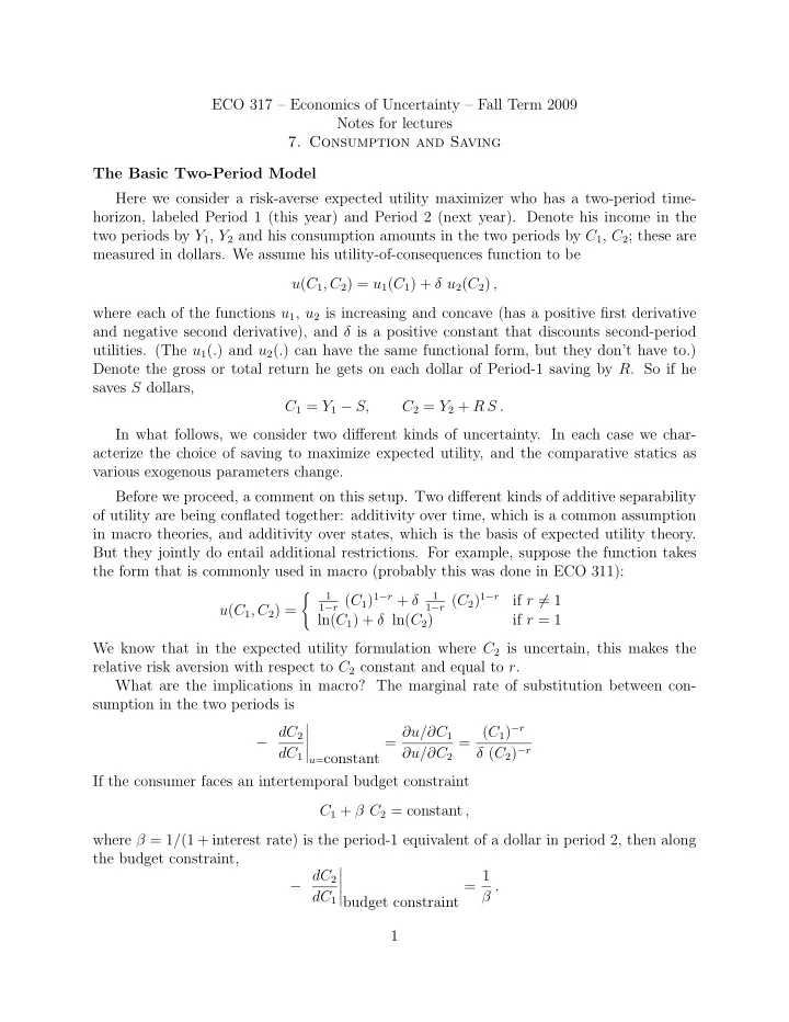
ECO 317 – Economics of Uncertainty – Fall Term 2009 Notes for lectures 7. Consumption and Saving The Basic Two-Period Model Here we consider a risk-averse expected utility maximizer who has a two-period time- horizon, labeled Period 1 (this year) and Period 2 (next year). Denote his income in the two periods by Y 1 , Y 2 and his consumption amounts in the two periods by C 1 , C 2 ; these are measured in dollars. We assume his utility-of-consequences function to be u ( C 1 , C 2 ) = u 1 ( C 1 ) + δ u 2 ( C 2 ) , where each of the functions u 1 , u 2 is increasing and concave (has a positive first derivative and negative second derivative), and δ is a positive constant that discounts second-period utilities. (The u 1 ( . ) and u 2 ( . ) can have the same functional form, but they don’t have to.) Denote the gross or total return he gets on each dollar of Period-1 saving by R . So if he saves S dollars, C 1 = Y 1 − S, C 2 = Y 2 + R S . In what follows, we consider two different kinds of uncertainty. In each case we char- acterize the choice of saving to maximize expected utility, and the comparative statics as various exogenous parameters change. Before we proceed, a comment on this setup. Two different kinds of additive separability of utility are being conflated together: additivity over time, which is a common assumption in macro theories, and additivity over states, which is the basis of expected utility theory. But they jointly do entail additional restrictions. For example, suppose the function takes the form that is commonly used in macro (probably this was done in ECO 311): 1 − r ( C 1 ) 1 − r + δ � 1 − r ( C 2 ) 1 − r 1 1 if r � = 1 u ( C 1 , C 2 ) = ln( C 1 ) + δ ln( C 2 ) if r = 1 We know that in the expected utility formulation where C 2 is uncertain, this makes the relative risk aversion with respect to C 2 constant and equal to r . What are the implications in macro? The marginal rate of substitution between con- sumption in the two periods is � = ( C 1 ) − r − dC 2 = ∂u/∂C 1 � � δ ( C 2 ) − r dC 1 � ∂u/∂C 2 u = constant � If the consumer faces an intertemporal budget constraint C 1 + β C 2 = constant , where β = 1 / (1 + interest rate) is the period-1 equivalent of a dollar in period 2, then along the budget constraint, � − dC 2 = 1 � β . � dC 1 � � budget constraint 1

For optimality, ( C 1 ) − r δ ( C 2 ) − r = 1 β , or � δ � 1 /r C 2 = . C 1 β Therefore 1 /r is the elasticity of substitution between first-period and second-period con- sumption. But r is also the coefficient of relative risk aversion, so 1 /r is also a quantitative measure of substitution across states of nature. Thus r is playing a dual role, and in principle there seems no reason why risk aversion (substituion across states) and substitution across time should be so tied together. More general formulations can allow separate parameters for the two; you will get them in more advanced courses. Uncertain Future Income Suppose there is uncertainty about future income, so Y 2 is a random variable with a density function f ( Y 2 ). The rate of return R is not random. The consumer chooses S to maximize expected utility. Assume in all that follows that the solution has S > 0. Expected utility, expressed as a function of the choice variable S , is given by EU ( S ) = E[ u 1 ( Y 1 − S ) + δ u 2 ( Y 2 + R S ) ] � = u 1 ( Y 1 − S ) + δ u 2 ( Y 2 + R S ) f ( Y 2 ) dY 2 . (1) Note: [1] The limits of integration (the support of Y 2 ) are omitted for brevity. [2] u 1 ( Y 1 − S ) is non-random and therefore its expectation is itself. [3] The multiplicative constant δ can be taken outside the expectation integral. It would not matter if you kept it inside the integration. The first-order condition is � EU ′ ( S ) = − u ′ u ′ 1 ( Y 1 − S ) + δ R 2 ( Y 2 + R S ) f ( Y 2 ) dY 2 = 0 , (2) where I have taken R outside the expectation integral becuase it is non-random here. The second-order condition is � 1 ( Y 1 − S ) + δ R 2 EU ′′ ( S ) = u ′′ u ′′ 2 ( Y 2 + R S ) f ( Y 2 ) dY 2 < 0 This is satisfied because u ′′ 1 , u ′′ 2 are both always negative. Equation (2) implicitly defines the optimal S . We consider its comparative statics. First suppose future income prospects become unambiguously better, in the sense that the distribution of Y 2 shifts to the right in the sense of first-order stochastic dominance (FOSD). From our general theory of comparative statics, we know that this will lead to a smaller optimal S if it lowers the whole function EU ′ ( S ). And the basic property of FOSD 2

shifts tells us that this will happen if u ′ 2 ( Y 2 + R S ) is a decreasing function of the random variable Y 2 for any given S . That is true because u ′′ 2 < 0. So we immediately have the result that an FOSD improvement in future income implies a less current saving. The intuition is as follows: The shift makes the person better off. Current consumption being a normal good, he wants more of it. Consuming more out of an unchanged current income lowers the saving. u '(Y +RS) 2 2 downward shift S Comparative statics of FOSD improvement in Y 2 Here we have another application of the general comparative statics argument, which you need to understand and later be able to do it correctly and instinctively. Next suppose future income becomes unambiguously riskier, that is, the distribution of Y 2 undergoes a mean-preserving spread in the sense of second-order stochastic dominance. This will raise the optimal S if it raises the expectation of u ′ 2 ( Y 2 + R S ) for each given R and S . We know that will happen if u ′ 2 ( Y 2 + R S ) is a convex function of Y 2 . The condition for this is u ′′′ 2 ( Y 2 + R S ) > 0. The textbook (p. 17) defines a measure of (absolute) prudence: P ( W ) = − u ′′′ ( W ) /u ′′ ( W ). Since u ′′ ( W ) < 0, we see that P ( W ) > 0 if u ′′′ ( W ) > 0. Qualitatively, we say that the decision-maker is prudent if P ( W ) > 0. We now see the reason for using this name more clearly: if the decision-maker is prudent, he saves more in preparation for a more uncertain propsect of future income. Uncertain Return to Saving The situation here is exactly the same as in the previous section, except that now Y 2 is non-random, and R is random with a density function g ( R ). The expected utility expressed as a function of S is EU ( S ) = E[ u 1 ( Y 1 − S ) + δ u 2 ( Y 2 + R S ) ] � = u 1 ( Y 1 − S ) + δ u 2 ( Y 2 + R S ) g ( R ) dR (3) The first-order condition is � EU ′ ( S ) = − u ′ u ′ 1 ( Y 1 − S ) + δ 2 ( Y 2 + R S ) R g ( R ) dR = 0 . (4) 3

Note that by contast with (2), now R is random and cannot be taken outside the expectation integral. The second-order condition is � 2 ( Y 2 + R S ) R 2 g ( R ) dR < 0 EU ′′ ( S ) = u ′′ 1 ( Y 1 − S ) + δ u ′′ This is satisfied because u ′′ 1 , u ′′ 2 are both always negative. A rightward shift of the distribution of R in the FOSD sense will increase EU ′ ( S ) at all S , and will therefore increase the optimal S , if u ′ 2 ( Y 2 + R S ) R is an increasing function of R for fixed Y 2 , S . The condition for this is u ′ 2 ( Y 2 + R S ) + u ′′ 2 ( Y 2 + R S ) S R > 0 . The left hand side of this inequality can be written as � � 1 + S R u ′′ 2 ( Y 2 + R S ) u ′ 2 ( Y 2 + R S ) u ′ 2 ( Y 2 + R S ) � � S R ( Y 2 + R S ) u ′′ 2 ( Y 2 + R S ) u ′ = 2 ( Y 2 + R S ) 1 + Y 2 + S R u ′ 2 ( Y 2 + R S ) S R � � u ′ = 2 ( Y 2 + R S ) 1 − Y 2 + S R ρ ( C 2 ) Since S R/ ( Y 2 + S R ) < 1, the coefficient of relative risk aversion being less than 1 is a sufficient condition to ensure that the whole expression is positive. If ρ is too high, then an FOSD improvement in the distribution of the rate of return on the risky asset can lead to a decrease in saving. Here the interpretation of 1 /ρ as the intertemporal elasticity of substitution comes useful. If ρ is large, this elasticity is small. Therefore there is only a small intertemporal substitution effect of the improvement in the rate of return, and it is overwhelmed by the income effect, which makes the consumer want to take out some of the benefit of this improved prospect in the form of today’s consumption. When the distribution of R undergoes a mean-preserving spread in the sense of second- order stochastic dominance, the expectation of u ′ 2 ( Y 2 + R S ) R rises for given Y 2 and S if u ′ 2 ( Y 2 + R S ) R is a convex function of R . If that is true, then for each S the mean-preserving spread of the distribution of R raises EU ′ ( S ), and by the same argument as above, the optimal S increases. Now d dR [ u ′ 2 ( Y 2 + R S ) R ] = u ′ 2 ( Y 2 + R S ) + u ′′ 2 ( Y 2 + R S ) S R , and d 2 2 ( Y 2 + R S ) S 2 R dR 2 [ u ′ u ′′ 2 ( Y 2 + R S ) S + u ′′ 2 ( Y 2 + R S ) S + u ′′′ 2 ( Y 2 + R S ) R ] = = S [ 2 u ′′ 2 ( Y 2 + R S ) + u ′′′ 2 ( Y 2 + R S ) S R ] We are told that S > 0, so the sign of the second derivative is the same as the sign of the expression in the bracket. The condition can be interpreted in terms of a measure of relative prudence, but it is not particularly useful. 4