E [ X ] = Roll a die n times. X ( ) Pr [ ] . X 1 + X 2 + + X n - PowerPoint PPT Presentation

CS70: Jean Walrand: Lecture 26. Random Variables: Review Expectation Definition: The expectation (mean, expected value) of a random Expectation; Geometric & Poisson Definition variable X is A random variable, X , for a random experiment with sample space Ω is a function X : Ω → ℜ . E [ X ] = ∑ a × Pr [ X = a ] . 1. Random Variables: Brief Review Thus, X ( · ) assigns a real number X ( ω ) to each ω ∈ Ω . a Indicator: 2. Expectation Definitions Let A be an event. The random variable X defined by For a ∈ ℜ , one defines X − 1 ( a ) := { ω ∈ Ω | X ( ω ) = a } . 3. Linearity of Expectation � 1 , if ω ∈ A X ( ω ) = 4. Geometric Distribution 0 , if ω / ∈ A The probability that X = a is defined as Pr [ X = a ] = Pr [ X − 1 ( a )] . 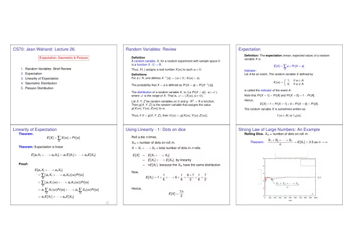5. Poisson Distribution is called the indicator of the event A . The distribution of a random variable X , is { ( a , Pr [ X = a ]) : a ∈ A } , Note that Pr [ X = 1 ] = Pr [ A ] and Pr [ X = 0 ] = 1 − Pr [ A ] . where A is the range of X . That is, A = { X ( ω ) , ω ∈ Ω } . Let X , Y , Z be random variables on Ω and g : ℜ 3 → ℜ a function. Hence, E [ X ] = 1 × Pr [ X = 1 ]+ 0 × Pr [ X = 0 ] = Pr [ A ] . Then g ( X , Y , Z ) is the random variable that assigns the value g ( X ( ω ) , Y ( ω ) , Z ( ω )) to ω . The random variable X is sometimes written as Thus, if V = g ( X , Y , Z ) , then V ( ω ) := g ( X ( ω ) , Y ( ω ) , Z ( ω )) . 1 { ω ∈ A } or 1 A ( ω ) . Linearity of Expectation Using Linearity - 1: Dots on dice Strong Law of Large Numbers: An Example Theorem: Rolling Dice. X m = number of dots on roll m . E [ X ] = ∑ Roll a die n times. X ( ω ) × Pr [ ω ] . X 1 + X 2 + ··· + X n ω Theorem: → E [ X 1 ] = 3 . 5 as n → ∞ . X m = number of dots on roll m . n Theorem: Expectation is linear X = X 1 + ··· + X n = total number of dots in n rolls. E [ a 1 X 1 + ··· + a n X n ] = a 1 E [ X 1 ]+ ··· + a n E [ X n ] . E [ X ] = E [ X 1 + ··· + X n ] = E [ X 1 ]+ ··· + E [ X n ] , by linearity Proof: = nE [ X 1 ] , because the X m have the same distribution E [ a 1 X 1 + ··· + a n X n ] Now, = ∑ ( a 1 X 1 + ··· + a n X n )( ω ) Pr [ ω ] E [ X 1 ] = 1 × 1 6 + ··· + 6 × 1 6 = 6 × 7 × 1 6 = 7 2 . ω 2 = ∑ ( a 1 X 1 ( ω )+ ··· + a n X n ( ω )) Pr [ ω ] ω Hence, = a 1 ∑ X 1 ( ω ) Pr [ ω ]+ ··· + a n ∑ X n ( ω ) Pr [ ω ] E [ X ] = 7 n ω ω 2 . = a 1 E [ X 1 ]+ ··· + a n E [ X n ] .

Y X Using Linearity - 2: Fixed point. Using Linearity - 3: Binomial Distribution. Using Linearity - 4 Hand out assignments at random to n students. Flip n coins with heads probability p . X - number of heads X = number of students that get their own assignment back. Binomial Distibution: Pr [ X = i ] , for each i . Assume A and B are disjoint events. Then 1 A ∪ B ( ω ) = 1 A ( ω )+ 1 B ( ω ) . X = X 1 + ··· + X n where � n � Taking expectation, we get p i ( 1 − p ) n − i . Pr [ X = i ] = X m = 1 { student m gets his/her own assignment back } . i Pr [ A ∪ B ] = E [ 1 A ∪ B ] = E [ 1 A + 1 B ] = E [ 1 A ]+ E [ 1 B ] = Pr [ A ]+ Pr [ B ] . One has � n � E [ X ] = ∑ i × Pr [ X = i ] = ∑ p i ( 1 − p ) n − i . i × E [ X ] = E [ X 1 + ··· + X n ] i i i = E [ X 1 ]+ ··· + E [ X n ] , by linearity In general, 1 A ∪ B ( ω ) = 1 A ( ω )+ 1 B ( ω ) − 1 A ∩ B ( ω ) . Uh oh. ... Or... a better approach: Let = nE [ X 1 ] , because all the X m have the same distribution � 1 Taking expectation, we get Pr [ A ∪ B ] = Pr [ A ]+ Pr [ B ] − Pr [ A ∩ B ] . if i th flip is heads = nPr [ X 1 = 1 ] , because X 1 is an indicator X i = 0 otherwise = n ( 1 / n ) , because student 1 is equally likely Observe that if Y ( ω ) = b for all ω , then E [ Y ] = b . E [ X i ] = 1 × Pr [“ heads ′′ ]+ 0 × Pr [“ tails ′′ ] = p . to get any one of the n assignments Thus, E [ X + b ] = E [ X ]+ b . = 1 . Moreover X = X 1 + ··· X n and Note that linearity holds even though the X m are not E [ X ] = E [ X 1 ]+ E [ X 2 ]+ ··· E [ X n ] = n × E [ X i ]= np . independent (whatever that means). Calculating E [ g ( X )] An Example Calculating E [ g ( X , Y , Z )] Let Y = g ( X ) . Assume that we know the distribution of X . Let X be uniform in {− 2 , − 1 , 0 , 1 , 2 , 3 } . We have seen that E [ g ( X )] = ∑ x g ( x ) Pr [ X = x ] . We want to calculate E [ Y ] . Let also g ( X ) = X 2 . Then (method 2) Using a similar derivation, one can show that Method 1: We calculate the distribution of Y : E [ g ( X , Y , Z )] = ∑ 3 g ( x , y , z ) Pr [ X = x , Y = y , Z = z ] . Pr [ Y = y ] = Pr [ X ∈ g − 1 ( y )] where g − 1 ( x ) = { x ∈ ℜ : g ( x ) = y } . x 2 1 ∑ E [ g ( X )] = x , y , z 6 x = − 2 This is typically rather tedious! An Example. Let X , Y be as shown below: { 4 + 1 + 0 + 1 + 4 + 9 } 1 6 = 19 Method 2: We use the following result. = 6 . Theorem: Method 1 - We find the distribution of Y = X 2 : E [ g ( X )] = ∑ g ( x ) Pr [ X = x ] . 0 . 2 0 . 3 1 x w.p. 2 8 (0 , 0) , w.p. 0 . 1 Proof:  4 , > > 6 (1 , 0) , w.p. 0 . 4 <  ( X , Y ) = w.p. 2  = ∑ g ( X ( ω )) Pr [ ω ] = ∑ 1 , (0 , 1) , w.p. 0 . 2 ∑  E [ g ( X )] g ( X ( ω )) Pr [ ω ] Y = 6 > > : (1 , 1) , w.p. 0 . 3 w.p. 1 0 , ω x ω ∈ X − 1 ( x ) 0 . 1 0 . 4 6  0  w.p. 1 = ∑ g ( x ) Pr [ ω ] = ∑  9 , 6 . ∑ ∑ g ( x ) Pr [ ω ] 0 1 x x ω ∈ X − 1 ( x ) ω ∈ X − 1 ( x ) E [ cos ( 2 π X + π Y )] = 0 . 1cos ( 0 )+ 0 . 4cos ( 2 π )+ 0 . 2cos ( π )+ 0 . 3cos ( 3 π ) = ∑ Thus, g ( x ) Pr [ X = x ] . E [ Y ] = 42 6 + 12 6 + 01 6 + 91 6 = 19 = 0 . 1 × 1 + 0 . 4 × 1 + 0 . 2 × ( − 1 )+ 0 . 3 × ( − 1 ) = 0 . x 6 .

X X µ Center of Mass Monotonicity Uniform Distribution Definition The expected value has a center of mass interpretation: Let X , Y be two random variables on Ω . We write X ≤ Y if X ( ω ) ≤ Y ( ω ) for all ω ∈ Ω , and similarly for X ≥ Y and X ≥ a Roll a six-sided balanced die. Let X be the number of pips 0 . 5 0 . 5 0 . 7 0 . 3 for some constant a . (dots). Then X is equally likely to take any of the values Facts { 1 , 2 ,..., 6 } . We say that X is uniformly distributed in 0 1 0 1 0 . 7 (a) If X ≥ 0, then E [ X ] ≥ 0. { 1 , 2 ,..., 6 } . 0 . 5 (b) If X ≤ Y , then E [ X ] ≤ E [ Y ] . p 1 p 2 p 3 More generally, we say that X is uniformly distributed in p n ( a n − µ ) = 0 Proof { 1 , 2 ,..., n } if Pr [ X = m ] = 1 / n for m = 1 , 2 ,..., n . a 2 a 3 n (a) If X ≥ 0 , every value a of X is nonnegative. Hence, a 1 ⇔ µ = a n p n = E [ X ] In that case, p 1 ( a 1 − µ ) n E [ X ] = ∑ p 3 ( a 3 − µ ) aPr [ X = a ] ≥ 0 . p 2 ( a 2 − µ ) n n m × 1 n = 1 n ( n + 1 ) = n + 1 ∑ ∑ a E [ X ] = mPr [ X = m ] = . n 2 2 m = 1 m = 1 (b) X ≤ Y ⇒ Y − X ≥ 0 ⇒ E [ Y ] − E [ X ] = E [ Y − X ] ≥ 0 . Example: B = ∪ m A m ⇒ 1 B ( ω ) ≤ ∑ m 1 A m ( ω ) ⇒ Pr [ ∪ m A m ] ≤ ∑ m Pr [ A m ] . Geometric Distribution Geometric Distribution Geometric Distribution Let’s flip a coin with Pr [ H ] = p until we get H . Pr [ X = n ] = ( 1 − p ) n − 1 p , n ≥ 1 . Pr [ X = n ] = ( 1 − p ) n − 1 p , n ≥ 1 . Note that ∞ ∞ ∞ ∞ ( 1 − p ) n − 1 = p ∑ ∑ ( 1 − p ) n − 1 p = p ∑ ∑ ( 1 − p ) n . Pr [ X n ] = For instance: n = 1 n = 1 n = 1 n = 0 ω 1 = H , or n = 0 a n = Now, if | a | < 1, then S := ∑ ∞ 1 1 − a . Indeed, ω 2 = T H , or 1 + a + a 2 + a 3 + ··· S = ω 3 = T T H , or a + a 2 + a 3 + a 4 + ··· = aS ω n = T T T T ··· T H . 1 + a − a + a 2 − a 2 + ··· = 1 . ( 1 − a ) S = Note that Ω = { ω n , n = 1 , 2 ,... } . Let X be the number of flips until the first H . Then, X ( ω n ) = n . Hence, ∞ 1 Also, ∑ Pr [ X n ] = p 1 − ( 1 − p ) = 1 . Pr [ X = n ] = ( 1 − p ) n − 1 p , n ≥ 1 . n = 1