SLIDE 1
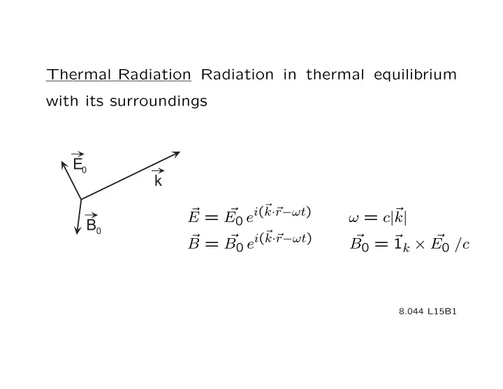
Thermal Radiation Radiation in thermal equilibrium with its surroundings E k E r = r
i(r k·r r−t)
= c|r k| E0 e B0 r r
i(r k·r r−t)
r r r B = B0 e B0 = 1k × E0 /c
8.044 L15B1
SLIDE 2 1
Time average energy density u = E0|E
2
Time average energy flux
1k Time average pressure (⇒ to - k) P = u Thermal radiation has a continuous distribution of frequencies.
u(ν,T)
Peaks near hν = 3kBT (h/kB 5 × 10⁻¹¹ K-sec)
ν
8.044 L15B2
SLIDE 3 Spectral Region ν (Hz) T (K) Thermal Rad. Radio Microwave Infrared Visible Ultraviolet X ray γ ray 106 1010 1013
1 2 × 10¹⁵
1016 1018 1021 1.7 × 10⁻⁵ 0.17 1.7 × 10² 8.5 × 10³ 1.7 × 10⁵ 1.7 × 10⁷ 1.7 × 10¹⁰ cosmic background room temp. sun’s surface black holes
8.044 L15B3
SLIDE 4 ENERGY ABSORBED ABSORPTIVITY α( ν,T) ENERGY INCIDENT
ISOTROPIC
ENERGY EMITTED EMISSIVE POWER e( ν,T) AREA
ISOTROPIC
8.044 L15B4
SLIDE 5 THERMAL RADIATION: PROPERTIES
2 ENERGY FLUXES, IN AND OUT OF CAVITY B FILTER: FREQUENCY OR POLARIZATION CAVITY A CAVITY B
TA TB
ASSUME TA = TB AND THERMAL EQUILIBRIUM
8.044 L15B5
SLIDE 6 CONCLUSIONS:
- u(ν, T ) is independent of shape and wall material
- u(ν, T ) is isotropic
- u(ν, T ) is unpolarized
8.044 L15B6
SLIDE 7 CONSIDER AN OBJECT IN THE CAVITY, IN THERMAL EQUILIBRIUM
dA T
COMPUTE THE ENERGY FLUX n
∆A
c∆t
θ
8.044 L15B7
SLIDE 8
∆E = (E in cylinder) p(θ, φ) dθ dφ sin θ 1 = (u ∆A cos θ c∆t) dθ dφ 2 2π
π/2 cos θ sin θ 2π 1
= c u ∆A ∆t dθ dφ 2 2π
1/4 1
1
⇒ energy flux onto dA = 4c u(ν, T )
8.044 L15B8
SLIDE 9
Momentum Flux Plane wave momentum density p r = u r 1k
c
|∆p| = 2|p⇒| since r −r p⇒ in = p⇒ out
8.044 L15B9
SLIDE 10
2 cos θ |∆p|ν = (E in cylinder) p(θ, φ) dθ dφ c
π/2 2π 1
= u(ν, T ) ∆A ∆t cos2 θ sin θ dθ dφ 2π
1/3 1
1
=
3u(ν, T ) ∆A ∆t
⇒ P (T ) = 1
u(ν, T ) dν
3
8.044 L15B10
SLIDE 11
Apply detailed balance to the object in the cavity. Eout = Ein e dA = α (4
1c u(ν, T )) dA
e(ν, T )
1
⇒ =
4c u(ν, T )
α(ν, T ) This ratio has a universal form for all materials. The result is known as KIRCHOFF’S LAW.
8.044 L15B11
SLIDE 12
Black Body Radiation If α ≡ 1 ≡ “Black” Then e(ν, T ) = 1
4c u(ν, T )
OVEN CAVITY AT T
Measure e(ν, T ) and obtain u(ν, T )
8.044 L15B12
SLIDE 13
Thermodynamic Approach
∞
u(T ) ≡ u(ν, T ) dν Then E(T, V ) = u(T )V
1
P (T, V ) = 3u(T )
8.044 L15B13
SLIDE 14
- This is enough to allow us to find u(T).
dE = TdS − PdV ∂E ∂S ∂P = T − P = T − P ∂V
T
∂V
T
∂T
V
1
= Tu(T) − 1
3u(T) 3
also = u(T)
T u(T) = AT 4
8.044 L15B14
SLIDE 15
Emissive Power of a Black (α = 1) Body e(ν, T ) = 1
4c u(ν, T ) ⇒ e(T ) = 1 4c u(T ) = 1AcT 4 4
e(T ) ∞ σT
4
This is known as the STEFAN-BOLTZMANN LAW. σ = 56.7 × 10⁻⁹ watts/m2K4
8.044 L15B15
SLIDE 16
r Statistical Mechanical Approach H? Single normal mode (plane standing wave) in a rectangular conducting cavity.
Ex z L
E r (r r, t) = E(t) sin(nπz/L)r 1x
0,0,n,r 1x
B (r r, t) = (nπc2/L)−1E ˙ (t) cos(nπz/L)r 1y
0,0,n,r 1y
8.044 L15B16
SLIDE 17 Energy density = 1E0E
µ 1
0 B
r or t average] 2 2
H = V 1E0E2(t) + 1 1 (nπc2/L)−2E ˙ 2(t)
2 2
2 µ0 V E0 = E2(t) + (nπc/L)−2 E ˙ 2(t) 2 2 Each mode corresponds to a harmonic oscillator.
8.044 L15B17
SLIDE 18
it
r Enx,ny,nz = |E|r j sin(nxπx/L) sin(nyπy/L) sin(nzπz/L)e The unit polarization vector E j has 2 possible orthog-
- nal directions and ni = 1, 2, 3 · · ·.
2
2 E E
2 E
πc
2 2 2
− c 2E = 0
(n + n + n )
x y z
t2 L
8.044 L15B18
SLIDE 19
- If the radian frequency < ω
nz R
L
2 2 2
R = n + n + n = ω
x y z
πc # modes (freq. < ω)
ny
1 4
GRID SPACING
= 2 × 8 × 3πR3
1 UNIT
3
π L
nx
= 3
πc
ω3
8.044 L15B19
SLIDE 20
d# L V D(ω) = = π ω2 = ω2 dω πc π2c3
D(ω)
ω
8.044 L15B20
SLIDE 21
Classical Statistical Mechanics D() kBT < E() >= kBT u(, T) =< E() > =
3 2
V π2c
∞
u(T) = u(, T) d = ∞ u(ω, T)
8.044 L15B21
CLASSICAL MEASURED
ω
SLIDE 22
Quantum Statistical Mechanics ¯ h < E() >= + ¯ h/2
¯ h/kT − 1
e D() ¯ h 3 u(, T ) =< E() > = + z. p. term π2c3
¯ h/kT − 1
V e du(, T ) To find the location of the maximum, set = 0. d The maximum occurs at ¯ h/kT ≈ 2.82.
8.044 L15B22
SLIDE 23
SLIDE 24
hω/2kT (1 − e −¯ hω/kT )−1
Z = Zi Zi = e
states i
The first factor in the expression for Zi comes from the zero-point energy. F (V, T ) = −kT ln Z = −kT ln Zi
states i
= −kT D(ω) [ln Zi] dω
8.044 L15B23
SLIDE 25
hω/kT )
F (V, T ) = −kT D(ω) − ln(1 − e dω + · · ·
−¯ hω/kT ) dω
= ω2 ln(1 − e π2c3
= (kT )4 x
2 ln(1 − e −x) dx
π2c3¯ h3
v- _
−π4
45
1 π2 = − (kT )4 V 45 c3¯ h3
8.044 L15B24
SLIDE 26
1 π2 P = − = (kT)4 ∂V T 45 (c¯ h)3 ∂F 4 π2 S = − = k4T 3 V ∂T V 45 (c¯ h)3 1 4 1 π2 E = F + TS = − + (· · ·) = (kT)4 V 45 45 15 (c¯ h)3 Note: P = 1
3 E/V = 1 3 u(T) independent of V .
8.044 L15B25
SLIDE 27 NOTE: THE ADIABATIC PATH IS T3V=CONSTANT
T
ADIABATIC T/T0 = (V/V0)-1 / 3
V
8.044 L15B26
SLIDE 28 MIT OpenCourseWare http://ocw.mit.edu
8.044 Statistical Physics I
Spring 2013 For information about citing these materials or our Terms of Use, visit: http://ocw.mit.edu/terms.