E Example l CSE 541 Numerical Methods Suppose we have three - - PowerPoint PPT Presentation

SLIDE 1

CSE 541 – Numerical Methods

Linear Systems y

E l Example

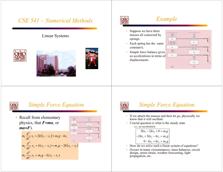
• Suppose we have three

masses all connected by i springs.

• Each spring has the same

constant k. constant k.

• Simple force balance gives

us accelerations in terms of di l displacements.

S l F E Simple Force Equation

• Recall from elementary

physics that F=ma or

( )

2

d

physics, that F ma, or ma=F).

( ) ( )

2 ) ( 2

2 1 1 1 2 1 2 1

k k d kx g m x x k x dt d m − + − =

( )

) ( 2 ) (

2 1 2 2 2 3 2 2 2

x x k g m x d m x x k g m x x k x dt d m − − + − = ) (

2 3 3 3 2 3

x x k g m x dt m − − =

S l F E Simple Force Equation

• If we attach the masses and then let go, physically we

know that it will oscillate

• Crucial question is what is the steady state

Crucial question is what is the steady state

– i.e., no acceleration

1 2 1

3 2 kx kx m g − + =

1 2 3 2 2 3 3

2 3 kx kx kx m g kx kx m g − + − = − + =

• How do we solve such a linear system of equations?
• Occurs in many circumstances: mass balances, circuit

design, stress-strain, weather forecasting, light i propagation, etc.

SLIDE 2

S f E Systems of Equations

• This simple example produces 3 equations in three unknowns:
• Geometrically this represents 3 planes in space.

S f E Systems of Equations

• Three different things can happen:

– Planes intersect at a single point. – A unique solution to the system of equations.

S f E Systems of Equations

• Planes do not intersect at all: (At least two

are parallel).

parallel planes

S f E Systems of Equations

• Planes intersect at an infinite number of

points (plane or line).

SLIDE 3

S f E Systems of Equations

• How do we know whether a unique solution

exists?

• How do we find such a solution?

S f E Systems of Equations

• In general, we may have n equations in n

unknowns unknowns.

• Can we find a solution?

C l ith t ffi i tl

• Can we program an algorithm to efficiently

find a solution?

• Is it well behaved? Accuracy?

Convergence? Stability?

Wh M ? What is a Matrix?

• A matrix is a set of elements, organized into

rows and columns rows and columns

⎤ ⎡ b

rows ⎤ ⎡

⎥ ⎤ ⎢ ⎡ b a

columns

[ ]

⎥ ⎥ ⎥ ⎤ ⎢ ⎢ ⎢ ⎡ = =

n n mxn ij

a a a a a a a A ... ...

2 22 21 1 12 11

⎥ ⎦ ⎢ ⎣ d c

⎥ ⎥ ⎦ ⎢ ⎢ ⎣

mn m m mxn j

a a a ...

2 1

M D f Matrix Definitions

• n x m Array of Scalars (n Rows and m Columns)

– n: row dimension of a matrix, m: column dimension , – m = n square matrix of dimension n – Element { }

m j n i aij , , 1 , , , 1 , K K = =

{ }

j

ij

[ ]

ij

a = A

SLIDE 4

M D f Matrix Definitions

• Column Matrices and Row Matrices

– Column matrix (n x 1 matrix): ( )

[ ]

⎥ ⎥ ⎤ ⎢ ⎢ ⎡ b b b

2 1

b

[ ]

⎥ ⎥ ⎥ ⎦ ⎢ ⎢ ⎢ ⎣ = =

n i

b b M b

– Row matrix (1 x n matrix): a = [ai] = [a1 a2 … an]

⎦ ⎣

n

B M O Basic Matrix Operations

• Addition (just add each element)

– Each matrix must be the same size! – Each matrix must be the same size!

⎤ ⎡ + + ⎤ ⎡ ⎤ ⎡ f b e a f e b a

[ ]

ij ij

b a + = + = B A C

• Properties of Matrix-Matrix Addition

⎥ ⎦ ⎤ ⎢ ⎣ ⎡ + + = ⎥ ⎦ ⎤ ⎢ ⎣ ⎡ + ⎥ ⎦ ⎤ ⎢ ⎣ ⎡ h d g c f h g f d c

• Properties of Matrix-Matrix Addition

– Commutative: Associative:

A B B A + = +

( ) ( )

C B A C B A + + = + +

– Associative:

( ) ( )

C B A C B A + + = + +

B M O Basic Matrix Operations

• Subtraction

⎤ ⎡ ⎤ ⎡ ⎤ ⎡ ⎥ ⎦ ⎤ ⎢ ⎣ ⎡ − − − − = ⎥ ⎦ ⎤ ⎢ ⎣ ⎡ − ⎥ ⎦ ⎤ ⎢ ⎣ ⎡ h d g c f b e a h g f e d c b a ⎦ ⎣ ⎦ ⎣ ⎦ ⎣

B M O Basic Matrix Operations

• Scalar-Matrix Multiplication

[ ]

a α α = A

[ ]

ij

a α α = A

• Properties of Scalar-Matrix Multiplication

( ) ( )A

A αβ β α =

( ) ( )

A A A A βα αβ αβ β α =

SLIDE 5

B M O Basic Matrix Operations

• Matrix-Matrix Multiplication

– A: n x l matrix B: l x m C: n x m matrix – A: n x l matrix, B: l x m C: n x m matrix

[ ]

= =

ij

c AB C

l

∑

=

=

l k kj ik ij

b a c

1

– example

⎥ ⎦ ⎤ ⎢ ⎣ ⎡ + + + + = ⎥ ⎦ ⎤ ⎢ ⎣ ⎡ ⎥ ⎦ ⎤ ⎢ ⎣ ⎡ dh cf dg ce bh af bg ae h g f e d c b a ⎦ ⎣ + + ⎦ ⎣ ⎦ ⎣ dh cf dg ce h g d c

M M l l Matrix Multiplication

Matrices A and B have these dimensions:

[n x m] and [p x q] [n x m] and [p x q]

M M l l Matrix Multiplication

Matrices A and B can be multiplied if:

[ ] d [ ] [n x m] and [p x q] m = p

M M l l Matrix Multiplication

The resulting matrix will have the dimensions:

[ ] d [ ] [n x m] and [p x q] n x q

SLIDE 6

Computation: A x B = C

A = a11 a12 a21 a22 ⎡ ⎣ ⎢ ⎤ ⎦ ⎥

[2 x 2]

⎣ ⎦

B = b11 b12 b13 b b b ⎡ ⎣ ⎢ ⎤ ⎦ ⎥

[2 x 3]

b21 b22 b23 ⎣ ⎢ ⎦ ⎥ ⎤ ⎡ + + +

23 12 13 11 22 12 12 11 21 12 11 11

b a b a b a b a b a b a ⎥ ⎦ ⎤ ⎢ ⎣ ⎡ + + + =

23 22 13 21 22 22 12 21 21 22 11 21

b a b a b a b a b a b a C

[2 x 3] [2 x 3]

Computation: A x B = C

2 3 ⎡ ⎤ A = 2 3 1 1 ⎡ ⎢ ⎤ ⎥ and B = 1 1 1 1 0 2 ⎡ ⎣ ⎢ ⎤ ⎦ ⎥ 1 0 ⎣ ⎢ ⎦ ⎥ 1 0 2 ⎣ ⎢ ⎦ ⎥

[3 x 2] [2 x 3]

A and B can be multiplied

⎥ ⎤ ⎢ ⎡ ⎥ ⎤ ⎢ ⎡ = + = + = + 8 2 5 8 2 * 3 1 * 2 2 * 3 1 * 2 5 1 * 3 1 * 2 ⎥ ⎥ ⎥ ⎦ ⎢ ⎢ ⎢ ⎣ = ⎥ ⎥ ⎥ ⎦ ⎢ ⎢ ⎢ ⎣ = + = + = + = + = + = + = 1 1 1 3 1 2 1 2 * 1 * 1 1 * 1 * 1 1 1 * 1 * 1 3 2 * 1 1 * 1 1 * 1 1 * 1 2 1 * 1 1 * 1 C

[3 x 3]

Computation: A x B = C Computation: A x B = C

2 3 ⎡ ⎤ A = 2 3 1 1 ⎡ ⎢ ⎢ ⎤ ⎥ ⎥ and B = 1 1 1 1 0 2 ⎡ ⎣ ⎢ ⎤ ⎦ ⎥ 1 0 ⎣ ⎢ ⎦ ⎥ 1 0 2 ⎣ ⎢ ⎦ ⎥

[3 x 2] [2 x 3]

⎥ ⎤ ⎢ ⎡ ⎥ ⎤ ⎢ ⎡ = + = + = + 8 2 5 8 2 * 3 1 * 2 2 * 3 1 * 2 5 1 * 3 1 * 2

Result is 3 x 3

⎥ ⎥ ⎥ ⎦ ⎢ ⎢ ⎢ ⎣ = ⎥ ⎥ ⎥ ⎦ ⎢ ⎢ ⎢ ⎣ = + = + = + = + = + = + = 1 1 1 3 1 2 1 2 * 1 * 1 1 * 1 * 1 1 1 * 1 * 1 3 2 * 1 1 * 1 1 * 1 1 * 1 2 1 * 1 1 * 1 C

[3 x 3]

M t i M lti li ti Matrix Multiplication

• Is AB = BA? Maybe, but maybe not!

⎥ ⎤ ⎢ ⎡ + = ⎥ ⎤ ⎢ ⎡ ⎥ ⎤ ⎢ ⎡ ... bg ae f e b a ⎥ ⎤ ⎢ ⎡ + = ⎥ ⎤ ⎢ ⎡ ⎥ ⎤ ⎢ ⎡ ... fc ea b a f e ⎥ ⎦ ⎢ ⎣ = ⎥ ⎦ ⎢ ⎣ ⎥ ⎦ ⎢ ⎣ ... ... h g d c ⎥ ⎦ ⎢ ⎣ = ⎥ ⎦ ⎢ ⎣ ⎥ ⎦ ⎢ ⎣ ... ... d c h g

• Heads up: multiplication is NOT commutative!

SLIDE 7

M M l l Matrix Multiplication

• Properties of Matrix-Matrix Multiplication

( ) ( )C

AB BC A =

( ) ( )

BA AB C AB BC A ≠ =

Th Id M The Identity Matrix

• Identity Matrix, I, is a Square Matrix:

⎧ if 1 j i

⎥ ⎤ ⎢ ⎡ 1

[ ]

⎩ ⎨ ⎧ = = =

• therwise

if 1 , j i a a

ij ij

I

⎥ ⎥ ⎥ ⎦ ⎢ ⎢ ⎢ ⎣ = 1 1 I

• Properties of the Identity matrix:

– AI = A IA = A

⎦ ⎣

– Multiplying a matrix with the Identity matrix does not change the initial matrix.

V t O ti Vector Operations

• Vector: 1 x N matrix
• Interpretation: a line in

⎥ ⎤ ⎢ ⎡a r

N dimensional space

• Dot Product, Cross

⎥ ⎥ ⎥ ⎦ ⎢ ⎢ ⎢ ⎣ = b v r

Product, and Magnitude defined on vectors only

⎥ ⎦ ⎢ ⎣c

y v x

M T Matrix Transpose

• Transpose: interchanging the rows and columns of

a matrix.

[ ]

ji T

a = A

• Properties of the Transpose
• (AT)T = A

( )

• (A + B) T = AT + BT
• (AB) T = BT AT

SLIDE 8

I f M Inverse of a Matrix

• Some matrices have an inverse, such that:

AA-1 = I, and A-1A = I ,

• By definition:

I-1 = I, since I-1I = I-1

• Inversion is tricky:

(ABC)-1 = C-1B-1A-1 Derived from non-commutativity property

D t i t f M t i Determinant of a Matrix

⎤ ⎡ b

• Used for inversion
• If det(A) = 0, then A has

⎥ ⎦ ⎤ ⎢ ⎣ ⎡ = d c b a A

no inverse

• Can be found using

bc ad A − = ) det( factorials, pivots, and cofactors.

⎥ ⎦ ⎤ ⎢ ⎣ ⎡ − − − =

−

a c b d bc ad A 1

1

⎦ ⎣

C l f M O Complexity of Matrix Ops

• Consider a square matrix of nxn with N elements
• Matrix Addition

– N additions, so either O(N) or O(n2)

• Scalar-Matrix multiplication

N ddi i i h O(N) O( 2) – N additions, so either O(N) or O(n2)

• Matrix-Matrix multiplication

– Each element has a row-column dot product – Each element has a row-column dot product. – Each element => n multiplications and n-1 additions – Total is n3 multiplications and n3-n2 additions, O(n3)

S f L E System of Linear Equations

• If our system of equations is linear, then we

can write the system as a matrix times a can write the system as a matrix times a vector of the unknowns equal to the constant terms constant terms.

3 1 = x System

2 3 2 2 = + y x System

⎤ ⎡ ⎤ ⎡ ⎤ ⎡ 3 1 x

7 3 = y x

24 2 5 2 3 2 = − + y x y x

⎤ ⎡ ⎤ ⎡ ⎤ ⎡ 2 3 2 x

⎥ ⎦ ⎤ ⎢ ⎣ ⎡ = ⎥ ⎦ ⎤ ⎢ ⎣ ⎡ ⎥ ⎦ ⎤ ⎢ ⎣ ⎡ 7 3 1 1 y x

⎥ ⎦ ⎤ ⎢ ⎣ ⎡ = ⎥ ⎦ ⎤ ⎢ ⎣ ⎡ ⎥ ⎦ ⎤ ⎢ ⎣ ⎡ − 24 2 2 5 3 2 y x

SLIDE 9

S f L E System of Linear Equations

• Examples in three-dimensions

3 System 4 System 10 5 3 14 4 5 8 11 2 4 + + = − + = + − z y x z y x y 25 3 3 12 14 4 5 8 11 2 4

3 2 1 3 2 1

= − + = + − x x x x x x y ⎥ ⎤ ⎢ ⎡ ⎥ ⎤ ⎢ ⎡ ⎥ ⎤ ⎢ ⎡ − 14 11 4 5 8 1 2 4 x 10 5 3 = + + − z y x 25 3 3 12

3 2 1

= − + x x x ⎥ ⎤ ⎢ ⎡ ⎥ ⎤ ⎢ ⎡ ⎥ ⎤ ⎢ ⎡ − 14 11 4 5 8 1 2 4

1

x ⎥ ⎥ ⎥ ⎦ ⎢ ⎢ ⎢ ⎣ = ⎥ ⎥ ⎥ ⎦ ⎢ ⎢ ⎢ ⎣ ⎥ ⎥ ⎥ ⎦ ⎢ ⎢ ⎢ ⎣− − 10 14 5 1 3 4 5 8 z y ⎥ ⎥ ⎥ ⎦ ⎢ ⎢ ⎢ ⎣ = ⎥ ⎥ ⎥ ⎦ ⎢ ⎢ ⎢ ⎣ ⎥ ⎥ ⎥ ⎦ ⎢ ⎢ ⎢ ⎣ − − 25 14 3 3 12 4 5 8

3 2

x x

S f L E System of Linear Equations

• Each of these examples can be

expressed in a simple matrix form: expressed in a simple matrix form:

Ax b =

• Where A is a n n matrix x and b are

Ax b

• Where A is a nxn matrix, x and b are

nx1 column matrices (or vectors).

S l M Special Matrices

• Some matrices have special powers or

properties: properties:

– Symmetric matrix Diagonal matrix – Diagonal matrix – Lower Triangular matrix Upper Triangular matrix – Upper Triangular matrix – Banded matrix

S M Symmetric Matrices

• Symmetric matrix – elements are symmetric

about the diagonal about the diagonal.

{aij} = {aji} for all i,j a = a a =a etc a12 = a21, a33=a33, etc.

• Implies A is equal to its transpose.

A AT A = AT

SLIDE 10

D l M Diagonal Matrices

• A diagonal matrix has zero’s everywhere except

possibly along the diagonal.

⎤ ⎡

11

d

p y g g

{aij} = 0 for all i ≠ j.

⎥ ⎥ ⎥ ⎦ ⎤ ⎢ ⎢ ⎢ ⎣ ⎡ =

33 22 11

d d D

• Addition, scalar-matrix multiplication and matrix-

matrix multiplication among diagonal matrices

( )

preserves diagonal matrices.

C = AB {cij} = 0 i ≠ j; {cii} = {aiibii} O(n)

• All operations are only O(n).

L T l M Lower Triangular Matrix

• A lower-triangular matrix has a value of

zero for all elements above the diagonal zero for all elements above the diagonal.

{lij} = 0 i < j. ⎤ ⎡l L ⎥ ⎥ ⎥ ⎥ ⎤ ⎢ ⎢ ⎢ ⎢ ⎡ = l l l L

22 21 11

O M M L

• Can you solve the first equation?

⎥ ⎦ ⎢ ⎣

− nn nn n

l l l

1 1

L

U T l M Upper-Triangular Matrix

• A upper-triangular matrix has a value of

zero for all elements below the diagonal zero for all elements below the diagonal.

{uij} = 0 i > j. ⎤ ⎡ u u u L ⎥ ⎥ ⎥ ⎥ ⎤ ⎢ ⎢ ⎢ ⎢ ⎡ =

− n n n

u u u u u U

1 22 1 12 11

O M M L

• Can you solve the last equation?

⎥ ⎦ ⎢ ⎣

− nn n n

u

1

L

B d d M Banded Matrices

• A banded matrix has zeros as we move

away from the diagonal away from the diagonal.

{bij} = 0 i > j+b and i < j-b. ⎥ ⎤ ⎢ ⎡

b

b b b

1 12 11

L L ⎥ ⎥ ⎥ ⎥ ⎢ ⎢ ⎢ ⎢ b b

22 21

O O O O M M O O O ⎥ ⎥ ⎥ ⎥ ⎥ ⎢ ⎢ ⎢ ⎢ ⎢ =

bn b

b b b B

1

O O O O M M O O O O O O O

band-width b

⎥ ⎥ ⎦ ⎢ ⎢ ⎣

− − nn nn nb n n

b b b b

1 1

L L O O O O M