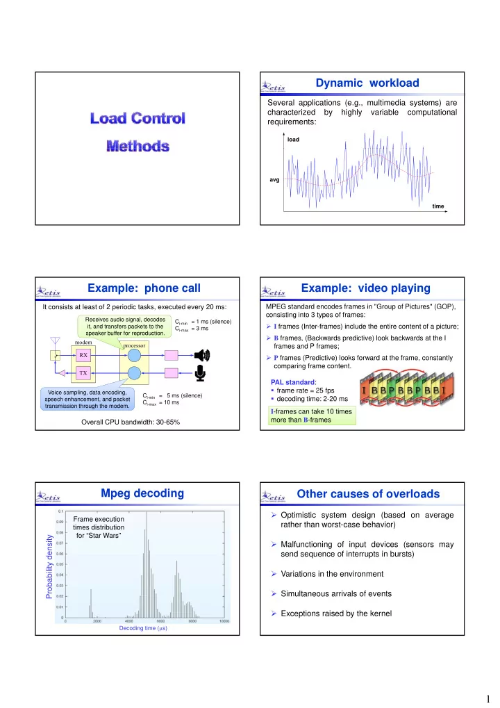
Dynamic workload Several applications (e.g., multimedia systems) - PDF document

Dynamic workload Several applications (e.g., multimedia systems) are characterized by highly variable computational requirements: load avg time Example: phone call Example: video playing It consists at least of 2 periodic tasks, executed every 20 ms: MPEG standard encodes frames in "Group of Pictures" (GOP), consisting into 3 types of frames: Receives audio signal, decodes C i-min = 1 ms (silence)  I frames (Inter-frames) include the entire content of a picture; it, and transfers packets to the C i-max = 3 ms speaker buffer for reproduction.  B frames, (Backwards predictive) look backwards at the I modem processor frames and P frames; RX RX  P frames (Predictive) looks forward at the frame, constantly comparing frame content. TX PAL standard :  frame rate = 25 fps Voice sampling, data encoding, C i-min = 5 ms (silence)  decoding time: 2-20 ms speech enhancement, and packet C i-max = 10 ms transmission through the modem. I -frames can take 10 times more than B -frames Overall CPU bandwidth: 30-65% Mpeg decoding Other causes of overloads  Optimistic system design (based on average Frame execution rather than worst-case behavior) times distribution for “Star Wars” density  Malfunctioning of input devices (sensors may send sequence of interrupts in bursts) Probability d  Variations in the environment  Simultaneous arrivals of events  Exceptions raised by the kernel Decoding time (  s) 1

Instantaneous load  (t) Load definitions Does not consider past or future activations, but     Soft aperiodic tasks: C only current jobs: n C      Hard periodic tasks: i U  1 T T  1 1 i i i i  2  Generic RT application:  3   if g ( t 1 , t 2 ) is the processor ( , ) g t t 0 2 4 6 8 10 12 14   max  1 2  t demand in [ t 1 , t 2 ], then:  ,   t t t t 1 2 2 1 Instantaneous load  (t) Example Maximum processor demand among those intervals from the current time and the deadlines of all active tasks.  1  1 (4) = 2/4 = 0.5 We can have at most one deadline for each active task  k ,  2  2 (4) = 5/6 = 0.83 hence:   ( ( ) ) c i t  3  3 i  (4)  3 (4) = 7/9 = 0.78 7/9 0 78    d d ( ) t i k 0 2 4 6 8 10 12 14 k   (4) = 0.83 d t  (t) k 1 0.5    ( ) max ( ) t t k k 0 2 4 6 8 10 12 14 Load and design assumptions A matter of cost  High predictability and low efficiency means System designed under System designed under worst-case assumptios average-case assumptios wasting resources  high cost load load – it can be justified only for very critical systems 1 1 0.75 0.75  High efficiency in resource usage requires a Hi h ffi i i i the system to: 0.5 0.5 – handle and tolerate overloads 0.25 0.25 – adapt for graceful degradation 0 0 – plan for exception handling mechanisms time time 2

Definitions Definitions Overrun: Situation in which a task exceeds its Overload: Situation in which  (t) > 1. expected utilization. Transient Overload Permanent Overload Execution Overrun  max > 1 but  avg  1  avg > 1 The task computation time exceeds its expected value:   1 1 0.75 0.75 Activation Overrun The next task activation occurs before its expected time: 0.5 0.5 0.25 0.25 expected interarrival time 0 0 time time Consequences of overruns Consequences of overruns A task overrun may not cause an overload: Consider the following applications with U < 1 :  1 1 8  1 overrun  2 (2/4) 0 2 4 6 8 10 12 12 12 20 20 4 4 8 8 16 16 24 24  2 But in general may delay the execution of other tasks, causing a deadline miss: (2/6) deadline miss 6 12 18 24  1  3 (1/12) 8 1  2 overrun 12 24 0 2 4 6 8 10 12 Consequences of overruns Example of overload In engine control, some tasks are activated at specific U < 1 but sporadic overruns can prevent  3 to run: angles of the crankshaft. The activation rate of these early completion execution overrun  1 tasks is proportional to the (2/4) angular velocity  of the engine: 12 12 20 20 4 4 8 8 16 16 24 24  2 t (2/6) C  6 12 18 24 u(  ) = 2   3 1 (1/12)  * = 2  12 24 C   * 3

Example of overload Load control methods engine task (high priority) Overrun handling Overload handling Function loss Car speed Resource Reservation Reactive vs. Proactive From now on Local vs. Global the car cannot decelerate! time Providing temporal isolation Transient overloads can be handled through Resource Reservation: a mechanism to bound the resource consumption of a task set to limit the interference caused to other tasks. To implement Resource Reservation we have to:  reserve a fraction of the processor bandwidth to a set of tasks;  prevent the task set to use more than the reserved fraction. Priorities vs. Reservations Resource Reservation Resource partition Resource enforcement  1  1  2  3 P 1 Prioritized READY QUEUE  2 10 % P 2 20 % Access  4  3  1 P 3  3  2 25 % 45 %  1 50%  A mechanism that prevents  1 = 0.5  1 a task to consume more Resource  2  2 30%  2 = 0.3 than its reserved amount. Reservation Each task receives a bandwidth  3  i  3 20% and behaves as it were  3 = 0.2  If a task executes more, it executing alone on a slower is delayed, preserving the processor of speed  i resource for other tasks. 4

Priorities vs. Reservations Benefits of Resource Reservation 1. Resource allocation is easier than priority mapping.  1 2. It provides temporal isolation: overruns occurring in Prioritized  2 Access a reservation do not affect other tasks.  3  Important for modularity and scalability p y y 3. Simpler schedulability analysis:  1 50%  Response times only depends on the application Resource  2 30% demand and the amount of reserved resource. Reservation  3 20% 4. Easier probabilistic approach Implementing RR Analysis under RR  1  1  1  1 server server  2b Ready queue  2b Ready queue  2  2 server CPU server CPU  2a  2a  3  3 scheduler scheduler  3   3  server server server server If a processor is partitioned into n reservations, we scheduler server must have that: n    Fixed priorities RM/DM Sporadic Server A U lub i  Dynamic priorities EDF 1 CBS i where A is the adopted scheduling algorithm. Types of reservations Soft CBS The original CBS formulation implements a SOFT HARD : when the budget is exhausted, the server is reservation: blocked until the next budget replenishment. In fact, more the Q s units can be executed in an interval P s if the processor is available. SOFT : when the budget is exhausted, the server P s P s remains active but at a lower priority level. 5 5  1 Note that Q s = 3  a HARD reservation (Q s , P s ) guarantees at most P s = 9 a budget Q s every period P s 0 3 6 9 12 15 18 21 24  a SOFT reservation (Q s , P s ) guarantees at least  2 a budget Q s every period P s 0 3 6 9 12 15 18 21 24 5

Problem with soft reservations Example with Hard CBS The deadline aging problem can be avoided by suspending the The use of idle times from a server can cause server when q s = 0 and recharging the budget at d s : irregular job executions and long delays: 16  1 P s P s P s P s P s 4 8 12 16 20 24 0  1 6 6 1 1 1 1 1 1 d 3 d 1 d 2 d 4 d 5 d 6 d 0  s 5 1 1 1 1 long delay Q s = 1 4 8 12 16 20 24 28 P s = 3 q s 0 3 6 9 12 15 18 21 24 10 0 2 4 6 8 10 12 14 16 18 20 22 24 26 28  2 0 3 6 9 12 15 18 21 24 CBS: Q s = 1, T s = 4 32 Hierarchical scheduling Hierarchical scheduling Resource reservation can be used to develop In general, a component can also be divided in other hierarchical systems, where each component is sub-components implemented within a reservation: Application 1 Application N Local Scheduler Local Scheduler Local Scheduler Local Scheduler Local Scheduler Local Scheduler       Component 1 Component N Component 1 Component N Global Scheduler Global Scheduler Computing Platform Computing Platform Hierarchical scheduling Hierarchical Analysis Global analysis : Servers must be schedulable by the global Global scheduler : the one managing the system ready queue scheduler running on the physical platform. Local schedulers : the ones managing the servers queues Local analysis : Applications must be scheduled by the local schedulers running on the components. Server S 4 Server S 1 Application 1 Application N   9   8   3  2    1    Local scheduler Local scheduler Local Scheduler Local Scheduler    Component 1 Component N S 4 S 3 S 2 S 1 CPU Global Scheduler Global scheduler Computing Platform 6