Dynamic programming Algorithm design technique A technique for - PowerPoint PPT Presentation

CS 3343 -- Spring 2009 Dynamic programming • Algorithm design technique • A technique for solving problems that have • overlapping subproblems • and, when used for optimization, have an optimal substructure property Dynamic Programming • Idea: Do not repeatedly solve the same subproblems, Carola Wenk but solve them only once and store the solutions in a Slides courtesy of Charles Leiserson with small dynamic programming table changes by Carola Wenk 3/17/09 CS 3343 Analysis of Algorithms 1 3/17/09 CS 3343 Analysis of Algorithms 2 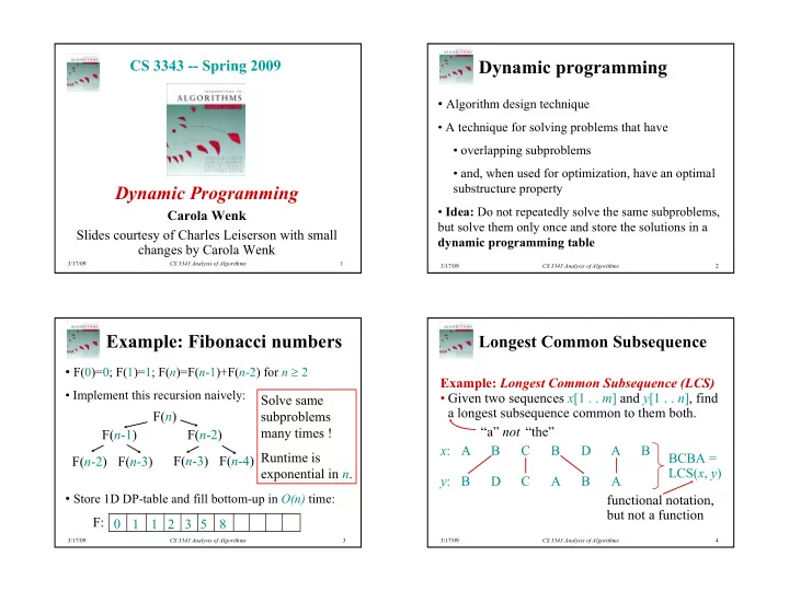Example: Fibonacci numbers Longest Common Subsequence • F(0)=0; F(1)=1; F( n )=F( n -1)+F( n -2) for n ≥ 2 Example: Longest Common Subsequence (LCS) • Implement this recursion naively: • Given two sequences x [1 . . m ] and y [1 . . n ], find Solve same a longest subsequence common to them both. F( n ) subproblems “a” not “the” many times ! F( n -1) F( n -2) x : A B C B D A B Runtime is BCBA = F( n -2) F( n -3) F( n -3) F( n -4) exponential in n . LCS( x , y ) y : B D C A B A • Store 1D DP-table and fill bottom-up in O(n) time: functional notation, but not a function F: 0 1 1 2 3 5 8 3/17/09 CS 3343 Analysis of Algorithms 3 3/17/09 CS 3343 Analysis of Algorithms 4 1

Brute-force LCS algorithm Towards a better algorithm Two-Step Approach: Check every subsequence of x [1 . . m ] to see 1. Look at the length of a longest-common if it is also a subsequence of y [1 . . n ]. subsequence. Analysis 2. Extend the algorithm to find the LCS itself. • 2 m subsequences of x (each bit-vector of Notation: Denote the length of a sequence s length m determines a distinct subsequence by | s | . of x ). Strategy: Consider prefixes of x and y . • Hence, the runtime would be exponential ! • Define c [ i , j ] = | LCS( x [1 . . i ], y [1 . . j ]) | . • Then, c [ m , n ] = | LCS( x , y ) | . 3/17/09 CS 3343 Analysis of Algorithms 5 3/17/09 CS 3343 Analysis of Algorithms 6 Recursive formulation Proof (continued) Theorem. Claim: z [1 . . k –1] = LCS( x [1 . . i –1], y [1 . . j –1]). c [ i –1, j –1] + 1 if x [ i ] = y [ j ], Suppose w is a longer CS of x [1 . . i –1] and c [ i , j ] = max { c [ i –1, j ], c [ i , j –1] } otherwise. y [1 . . j –1], that is, | w | > k –1. Then, cut and paste : w || z [ k ] ( w concatenated with z [ k ]) is a Proof. Case x [ i ] = y [ j ]: common subsequence of x [1 . . i ] and y [1 . . j ] 1 2 i m ... x : with | w || z [ k ] | > k . Contradiction, proving the = j 1 2 n claim. ... y : Thus, c [ i –1, j –1] = k –1, which implies that c [ i , j ] = c [ i –1, j –1] + 1. Let z [1 . . k ] = LCS( x [1 . . i ], y [1 . . j ]), where c [ i , j ] = k . Then, z [ k ] = x [ i ], or else z could be extended. Other cases are similar. Thus, z [1 . . k –1] is CS of x [1 . . i –1] and y [1 . . j –1]. 3/17/09 CS 3343 Analysis of Algorithms 7 3/17/09 CS 3343 Analysis of Algorithms 8 2

Dynamic-programming Recursive algorithm for LCS hallmark #1 LCS( x , y , i , j ) Optimal substructure if x [ i ] = y [ j ] An optimal solution to a problem then c [ i , j ] ← LCS( x , y , i –1, j –1) + 1 (instance) contains optimal else c [ i , j ] ← max { LCS( x , y , i– 1, j ), solutions to subproblems. LCS( x , y , i , j –1) } Recurrence Worst-case: x [ i ] ≠ y [ j ], in which case the algorithm evaluates two subproblems, each If z = LCS( x , y ), then any prefix of z is an LCS of a prefix of x and a prefix of y . with only one parameter decremented. 3/17/09 CS 3343 Analysis of Algorithms 9 3/17/09 CS 3343 Analysis of Algorithms 10 Dynamic-programming Recursion tree hallmark #2 m = 3, n = 4: 3,4 3,4 Overlapping subproblems A recursive solution contains a 2,4 3,3 same 2,4 3,3 subproblem “small” number of distinct m + n subproblems repeated many times. 1,4 2,3 2,3 3,2 1,4 2,3 2,3 3,2 1,3 2,2 1,3 2,2 1,3 2,2 1,3 2,2 The number of distinct LCS subproblems for two strings of lengths m and n is only mn . Height = m + n ⇒ work potentially exponential. , but we’re solving subproblems already solved! 3/17/09 CS 3343 Analysis of Algorithms 11 3/17/09 CS 3343 Analysis of Algorithms 12 3

Dynamic-programming Memoization algorithm Memoization: After computing a solution to a There are two variants of dynamic subproblem, store it in a table. Subsequent calls check the table to avoid redoing work. programming: for all i , j : c [ i ,0]=0 and c [0, j ]=0 LCS( x , y , i , j ) 1. Memoization if c [ i , j ] = NIL 2. Bottom-up dynamic programming then if x [ i ] = y [ j ] same (often referred to as “dynamic then c [ i , j ] ← LCS( x , y , i –1, j –1) + 1 as else c [ i , j ] ← max { LCS( x , y , i –1, j ), programming”) before LCS( x , y , i , j –1) } Time = Θ ( mn ) = constant work per table entry. Space = Θ ( mn ). 3/17/09 CS 3343 Analysis of Algorithms 13 3/17/09 CS 3343 Analysis of Algorithms 14 Memoization Recursive formulation 1 2 3 4 5 6 7 x : A B C B D A B c [ i –1, j –1] + 1 if x [ i ] = y [ j ], LCS( x , y ,7,6) c [ i , j ] = 0 0 0 0 0 0 0 0 max { c [ i –1, j ], c [ i , j –1] } otherwise. 0 0 0 0 0 0 0 0 y : (6,6) (7,5) 1 B 0 nil nil 0 nil nil nil nil nil nil nil nil 1 0 nil nil nil nil (5,5) (6,4) 2 D 0 nil nil nil nil 1 nil nil nil nil nil nil nil nil nil 0 0 nil c: i -1 i (4,5) 3 C 0 nil nil 0 nil nil nil nil nil nil nil nil nil nil (5,4) (5,3) 2 0 nil nil j -1 • • • 4 A 0 nil nil 1 nil nil nil nil nil nil nil nil nil nil nil 0 nil • • • • • • j c[ i , j ] c[ i , j ] 5 B 0 nil nil nil nil nil nil nil nil nil nil nil nil 2 0 nil nil 6 A 0 nil nil nil nil nil nil nil nil nil nil nil 0 nil nil nil 3/17/09 CS 3343 Analysis of Algorithms 15 3/17/09 CS 3343 Analysis of Algorithms 16 4

Bottom-up dynamic- Bottom-up dynamic- programming algorithm programming algorithm A B C B D A B A A B B C C B B D D A A B B I DEA : I DEA : Compute the Compute the 0 0 0 0 0 0 0 0 0 0 0 0 0 0 0 0 0 0 0 0 0 0 0 0 0 0 0 0 0 0 0 0 0 0 0 0 0 0 0 0 table bottom-up. table bottom-up. B 0 0 1 1 1 1 1 1 B B 0 0 1 1 1 1 1 1 1 0 0 1 1 1 1 1 1 0 0 1 1 1 1 1 1 1 Time = Θ ( mn ). Time = Θ ( mn ). D 0 0 1 1 1 2 2 2 D D 0 0 1 1 1 2 2 2 2 0 0 1 1 1 2 2 2 0 0 1 1 1 2 2 2 2 Reconstruct C 0 0 1 2 2 2 2 2 C C 0 0 1 2 2 2 2 2 2 0 0 1 2 2 2 2 2 0 0 1 2 2 2 2 2 2 LCS by back- A 0 1 1 2 2 2 3 3 A A 0 1 1 2 2 2 3 3 3 0 1 1 2 2 2 3 3 tracing. 0 1 1 2 2 2 3 3 3 Space = Θ ( mn ). B 0 1 2 2 3 3 3 4 B B 0 1 2 2 3 3 3 4 4 0 1 2 2 3 3 3 4 0 1 2 2 3 3 3 4 4 Exercise: A 0 1 2 2 3 3 4 4 A A 0 1 2 2 3 3 4 4 4 0 1 2 2 3 3 4 4 0 1 2 2 3 3 4 4 4 O (min{ m , n }). 3/17/09 CS 3343 Analysis of Algorithms 17 3/17/09 CS 3343 Analysis of Algorithms 18 5