Dynamic Programming 2/24/2005 1:46 AM Matrix Chain-Products Matrix - PDF document

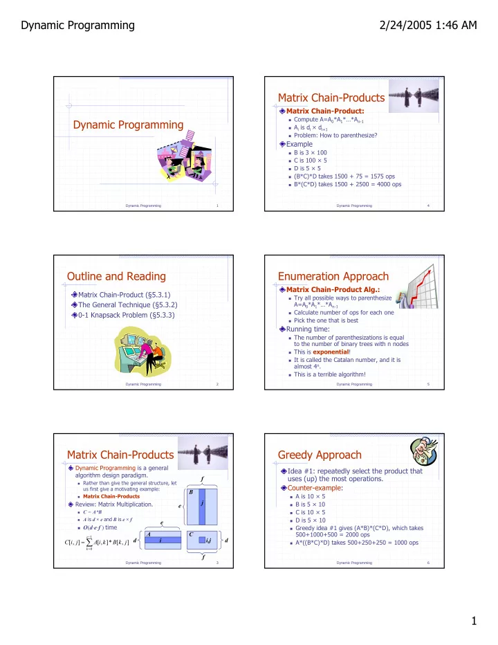
Dynamic Programming 2/24/2005 1:46 AM Matrix Chain-Products Matrix Chain-Product: � Compute A=A 0 *A 1 *…*A n-1 Dynamic Programming � A i is d i × d i+1 � Problem: How to parenthesize? Example � B is 3 × 100 � C is 100 × 5 � D is 5 × 5 � (B*C)*D takes 1500 + 75 = 1575 ops � B*(C*D) takes 1500 + 2500 = 4000 ops Dynamic Programming 1 Dynamic Programming 4 Outline and Reading Enumeration Approach Matrix Chain-Product Alg.: Matrix Chain-Product (§5.3.1) � Try all possible ways to parenthesize The General Technique (§5.3.2) A=A 0 *A 1 *…*A n-1 � Calculate number of ops for each one 0-1 Knapsack Problem (§5.3.3) � Pick the one that is best Running time: � The number of parenthesizations is equal to the number of binary trees with n nodes � This is exponential ! � It is called the Catalan number, and it is almost 4 n . � This is a terrible algorithm! Dynamic Programming 2 Dynamic Programming 5 Matrix Chain-Products Greedy Approach Dynamic Programming is a general Idea #1: repeatedly select the product that algorithm design paradigm. uses (up) the most operations. f � Rather than give the general structure, let Counter-example: us first give a motivating example: B � A is 10 × 5 � Matrix Chain-Products j Review: Matrix Multiplication. � B is 5 × 10 e � C is 10 × 5 � C = A * B � A is d × e and B is e × f � D is 5 × 10 e � O ( d ⋅ e ⋅ f ) time � Greedy idea #1 gives (A*B)*(C*D), which takes A C 500+1000+500 = 2000 ops e − 1 ∑ d i i,j d = C [ i , j ] A [ i , k ] * B [ k , j ] � A*((B*C)*D) takes 500+250+250 = 1000 ops k = 0 f Dynamic Programming 3 Dynamic Programming 6 1

Dynamic Programming 2/24/2005 1:46 AM Dynamic Programming Another Greedy Approach Algorithm Visualization Idea #2: repeatedly select the product that uses The bottom-up = + + N min { N N d d d } + + + the fewest operations. i , j i , k k 1 , j i k 1 j 1 construction fills in the i ≤ k < j N array by diagonals Counter-example: N 0 1 2 i j … n-1 N i,j gets values from � A is 101 × 11 0 previous entries in i-th 1 row and j-th column � B is 11 × 9 … answer Filling in each entry in � C is 9 × 100 i the N table takes O(n) � D is 100 × 99 time. � Greedy idea #2 gives A*((B*C)*D)), which takes Total run time: O(n 3 ) j 109989+9900+108900=228789 ops Getting actual � (A*B)*(C*D) takes 9999+89991+89100=189090 ops parenthesization can be done by remembering n-1 The greedy approach is not giving us the “k” for each N entry optimal value. Dynamic Programming 7 Dynamic Programming 10 Dynamic Programming “Recursive” Approach Algorithm Define subproblems : Since Algorithm matrixChain ( S ): subproblems � Find the best parenthesization of A i *A i+1 *…*A j . Input: sequence S of n matrices to be multiplied overlap, we don’t � Let N i,j denote the number of operations done by this use recursion. Output: number of operations in an optimal subproblem. Instead, we parenthesization of S construct optimal � The optimal solution for the whole problem is N 0,n-1 . for i ← 1 to n − 1 do subproblems Subproblem optimality : The optimal solution can be N i,i ← 0 “bottom-up.” defined in terms of optimal subproblems N i,i ’s are easy, so for b ← 1 to n − 1 do start with them { b = j − i is the length of the problem } � There has to be a final multiplication (root of the expression Then do tree) for the optimal solution. for i ← 0 to n − b − 1 do problems of � Say, the final multiply is at index i: (A 0 *…*A i )*(A i+1 *…*A n-1 ). j ← i + b “length” 2,3,… subproblems, � Then the optimal solution N 0,n-1 is the sum of two optimal N i,j ← +∞ and so on. subproblems, N 0,i and N i+1,n-1 plus the time for the last multiply. for k ← i to j − 1 do Running time: If the global optimum did not have these optimal N i,j ← min{ N i,j , N i,k + N k+ 1 ,j + d i d k+ 1 d j+ 1 } � O(n 3 ) subproblems, we could define an even better “optimal” return N 0, n − 1 solution. Dynamic Programming 8 Dynamic Programming 11 The General Dynamic Characterizing Equation Programming Technique The global optimal has to be defined in terms of Applies to a problem that at first seems to optimal subproblems, depending on where the final require a lot of time (possibly exponential), multiply is at. provided we have: Let us consider all possible places for that final multiply: � Simple subproblems: the subproblems can be � Recall that A i is a d i × d i+1 dimensional matrix. defined in terms of a few variables, such as j, k, l, � So, a characterizing equation for N i,j is the following: m, and so on. � Subproblem optimality: the global optimum value = + + N min { N N d d d } can be defined in terms of optimal subproblems + + + i , j i , k k 1 , j i k 1 j 1 i ≤ k < j � Subproblem overlap: the subproblems are not independent, but instead they overlap (hence, should be constructed bottom-up). Note that subproblems are not independent–the subproblems overlap . Dynamic Programming 9 Dynamic Programming 12 2

Dynamic Programming 2/24/2005 1:46 AM A 0/1 Knapsack Algorithm, The 0/1 Knapsack Problem Second Attempt Given: A set S of n items, with each item i having S k : Set of items numbered 1 to k. � w i - a positive weight Define B[k,w] to be the best selection from S k with � b i - a positive benefit weight at most w Goal: Choose items with maximum total benefit but with Good news: this does have subproblem optimality. weight at most W. If we are not allowed to take fractional amounts, then − > this is the 0/1 knapsack problem . ⎧ B [ k 1 , w ] if w w = k B [ k , w ] ⎨ � In this case, we let T denote the set of items we take − − − + max{ B [ k 1 , w ], B [ k 1 , w w ] b } else ⎩ k k ∑ b � Objective: maximize I.e., the best subset of S k with weight at most w is i i ∈ T either ∑ ≤ � the best subset of S k-1 with weight at most w or w W � Constraint: i � the best subset of S k-1 with weight at most w − w k plus item k i ∈ T Dynamic Programming 13 Dynamic Programming 16 Example 0/1 Knapsack Algorithm Given: A set S of n items, with each item i having ⎧ B [ k − 1 , w ] if w > w B [ k , w ] = k ⎨ − − − + � b i - a positive “benefit” ⎩ max{ B [ k 1 , w ], B [ k 1 , w w ] b } else k k � w i - a positive “weight” Algorithm 01Knapsack ( S, W ): Recall the definition of Input: set S of n items with benefit b i Goal: Choose items with maximum total benefit but with B[k,w] and weight w i ; maximum weight W weight at most W. Since B[k,w] is defined in Output: benefit of best subset of S with “knapsack” terms of B[k − 1,*], we can weight at most W use two arrays of instead of let A and B be arrays of length W + 1 a matrix for w ← 0 to W do Items: Running time: O(nW). B [ w ] ← 0 Not a polynomial-time for k ← 1 to n do box of width 9 in 1 2 3 4 5 algorithm since W may be copy array B into array A Solution: Weight: large 4 in 2 in 2 in 6 in 2 in for w ← w k to W do • item 5 ($80, 2 in) Benefit: This is a pseudo-polynomial if A [ w − w k ] + b k > A [ w ] then $20 $3 $6 $25 $80 • item 3 ($6, 2in) time algorithm B [ w ] ← A [ w − w k ] + b k • item 1 ($20, 4in) return B [ W ] Dynamic Programming 14 Dynamic Programming 17 A 0/1 Knapsack Algorithm, First Attempt S k : Set of items numbered 1 to k. Define B[k] = best selection from S k . Problem: does not have subproblem optimality: � Consider set S={(3,2),(5,4),(8,5),(4,3),(10,9)} of (benefit, weight) pairs and total weight W = 20 Best for S 4 : Best for S 5 : Dynamic Programming 15 3