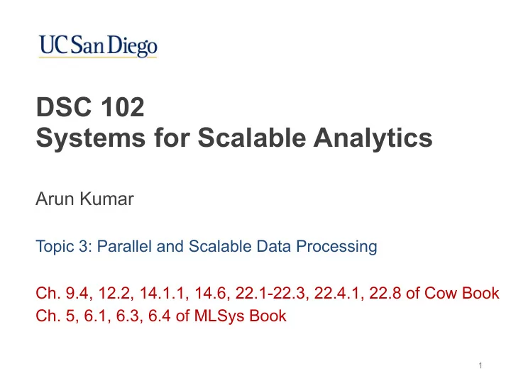
DSC 102 Systems for Scalable Analytics Arun Kumar Topic 3: - - PowerPoint PPT Presentation

Topic 3: Parallel and Scalable Data Processing

• Ch. 9.4, 12.2, 14.1.1, 14.6, 22.1-22.3, 22.4.1, 22.8 of Cow Book
• Ch. 5, 6.1, 6.3, 6.4 of MLSys Book

Arun Kumar

1

DSC 102
 Systems for Scalable Analytics

2

Q: Why bother with large-scale data? Why does sampling not suffice?

3

4

Large-Scale Data in Astronomy

High-res. images: ~200 GB per day since 2000 (1PB+) Astronomers can study complex galactic evolution behaviors

5

6

Large-Scale Data in Genomics

Precision Medicine is becoming a reality Analyze genomes across cohorts and prescribe targeted drugs and treatments ~3GB genome per human 900PB+ for USA

7

8

Large-Scale Data in E-commerce

Log all user behavior (views, clicks, pauses, searches, etc.) Recommender systems combine TBs of data from all users and movies to deliver a tailored experience

9

Large-Scale Data in Computer Vision

10million+ images labeled (20,000 classes) by crowdsourcing >500GB uncompressed as tensors Harbinger of deep learning revolution

10

“The Unreasonable Effectiveness of Data”

https://ai.googleblog.com/2017/07/revisiting-unreasonable-effectiveness.html

When prediction target complexity is high, more training data coupled with more complex models yield higher accuracy as number

• f training examples grows

11

Bias-Variance Tradeoff of ML

High Bias: Roughly, model is not rich enough to represent data High Variance: Model overfits to given data; poor generalization Large-scale training data lowers variance and raises accuracy!

12

Why Large-Scale Data?

❖ Large-scale data is a game changer for data science: ❖ Enables study of granular phenomena in sciences, businesses, etc. that were never before possible ❖ Enables fundamentally new applications and a high degree of personalization/customization ❖ Enables more complex ML prediction targets and mitigates variance to offer high accuracy ❖ Hardware has kept pace to power the above: ❖ Storage capacity has exploded (PB clusters) ❖ Compute capacity has grown (multi-core, GPUs, etc.) ❖ DRAM capacity has grown (10GBs to TBs) ❖ Cloud computing helps “democratize” access

13

“Big Data”

❖ Marketing term; think “Big” as in “Big Oil”, not “big building” ❖ Became popular in late 2000s to early 2010s ❖ Wikipedia says: “Data that is so large and complex that existing toolkits [read RDBMSs!] are not adequate” ❖ Typical characterization by 3 Vs: ❖ Volume: larger than single-node DRAM ❖ Variety: relations, docs, tweets, multimedia, etc. ❖ Velocity: high generation rate, e.g., sensors, surveillance

Why “Big Data” now? 1. Applications

❖ New “data-driven mentality” in almost all human endeavors: ❖ Web: search, e-commerce, e-mails, social media ❖ Science: satellite imagery, CERN’s LHC, document corpora ❖ Medicine: pharmacogenomics, precision medicine ❖ Logistics: sensors, GPS, “Internet of Things” ❖ Finance: high-throughput trading, monitoring ❖ Humanities: digitized books/literature, social media ❖ Governance: e-voting, targeted campaigns, NSA ☺ ❖ …

14

Why “Big Data” now? 2. Storage

15

16

To analyze large-scale data, parallel and scalable data systems are indispensable!

17

Outline

❖ Basics of Parallelism

❖ Task Parallelism ❖ Single-Node Multi-Core; SIMD; Accelerators

❖ Basics of Scalable Data Access

❖ Paged Access; I/O Costs; Layouts/Access Patterns ❖ Scaling Data Science Operations

❖ Data Parallelism: Parallelism + Scalability

❖ Data-Parallel Data Science Operations ❖ Optimizations and Hybrid Parallelism

18

Parallel Data Processing

Central Issue: Workload takes too long for one processor! Basic Idea: Split up workload across processors and perhaps also across machines/workers (aka “Divide and Conquer”) Key new concept in parallel processing: ❖ Threads: Generalization of process abstraction of OS ❖ A program/process can spawn many threads; each runs a part of the program’s computations simultaneously ❖ All threads share process address space (so, data too) ❖ In multi-core CPUs, a thread uses up 1 core ❖ “Hyper-threading”: Virtualizes a core to run 2 threads!

19

Multiple Threads in a Process

20

Parallel Data Processing

Central Issue: Workload takes too long for one processor! Basic Idea: Split up workload across processors and perhaps also across machines/workers (aka “Divide and Conquer”) Key new concept in parallel processing: ❖ DataFlow Graph: A directed graph representation of a program with vertices being abstract operations from a restricted set of computational primitives: ❖ Relational dataflows: RDBMS, Pandas ❖ Matrix/tensor dataflows: R, NumPy, TensorFlow, etc. ❖ Task Graph: Similar but coarse-grained; vertex is a process

21

Example Relational Dataflow Graph

Aka Logical Query Plan in the DB systems world Intermediate data Operators from extended relational algebra Input data

⇡((R) ∪ S . / T)

22

Example Tensor Dataflow Graph

ReLU (WX + b)

Input data Operators from LA/DL tool’s tensor algebra Intermediate data Aka Neural Computational Graph in the ML systems world

23

Example Task Graph

NB: Dask conflates the concepts of Dataflow and Task graphs because an “operation” on a Dask DataFrame becomes its own separate process/program under the covers!

https://docs.dask.org/en/latest/graphviz.html

❖ More coarse-grained than

• perator-level dataflows

❖ Vertex: A full task/process ❖ Edge: A dependency between tasks ❖ Directed Acyclic Graph model (DAG) common; cycles? ❖ Data may not be shown

24

Parallel Data Processing

Key parallelism paradigms in data systems: Central Issue: Workload takes too long for one processor! Basic Idea: Split up workload across processors and perhaps also across machines/workers (aka “Divide and Conquer”) Within a node: Across nodes: Shared Replicated Partitioned “SIMD” “Pipelining” Dataset is: “Task Parallel” Systems N/A “Data Parallel” Systems

25

Outline

❖ Basics of Parallelism

❖ Task Parallelism ❖ Single-Node Multi-Core; SIMD; Accelerators

❖ Basics of Scalable Data Access

❖ Paged Access; I/O Costs; Layouts/Access Patterns ❖ Scaling Data Science Operations

❖ Data Parallelism: Parallelism + Scalability

❖ Data-Parallel Data Science Operations ❖ Optimizations and Hybrid Parallelism

26

Task Parallelism

Basic Idea: Split up tasks across workers; if there is a common dataset that they read, just make copies of it (aka replication)

T1

D

T2 T3 T4 T5 T6

Example:

2) Put T1 on worker 1 (W1), T2 on W2, T3 on W3; run all 3 in parallel

This is your PA1 setup! Except, Dask Scheduler puts tasks on workers for you.

1) Copy whole D to all workers

Given 3 workers

3) After T1 ends, run T4 on W1; after T2 ends, run T5 on W2; after T3 ends, W3 is idle 4) After T4 & T5 end, run T6 on W1; W2 is idle

27

Task Parallelism

❖ Topological sort of tasks in task graph for scheduling ❖ Notion of a “worker” in task parallelism can be at processor/ core level, not just at node/server level ❖ Thread-level parallelism instead of process-level ❖ E.g., Dask: 4 worker nodes x 4 cores = 16 workers total ❖ Main pros of task parallelism: ❖ Simple to understand; easy to implement ❖ Independence of workers => low software complexity ❖ Main cons of task parallelism: ❖ Data replication across nodes; wastes memory/storage ❖ Idle times possible on workers Basic Idea: Split up tasks across workers; if there is a common dataset that they read, just make copies of it (aka replication)

28

Degree of Parallelism

❖ The largest amount of concurrency possible in the task graph, i.e., how many task can be run simultaneously

T1

D

T2 T3 T4 T5 T6

Example: Given 3 workers

Degree of parallelism is only 3 So, more than 3 workers is not useful for this workload!

Q: How do we quantify the performance benefits of task parallelism?

But over time, degree of parallelism keeps dropping in this example

29

Quantifying Benefit of Parallelism: Speedup

Speedup = Completion time given only 1 worker Completion time given n (>1) workers Q: But given n workers, can we get a speedup of n? It depends! (On degree of parallelism, task dependency graph structure, intermediate data sizes, etc.)

30

Quantifying Benefit of Parallelism

Number of workers Runtime speedup (fixed data size) 1 4 8 12 1 4 8 12 Linear Speedup Sublinear Speedup Q: Is superlinear speedup/scaleup ever possible? Factor (# workers, data size) Runtime speedup 1 4 8 12 1 0.5 2 Linear Scaleup Sublinear Scaleup Speedup plot / Strong scaling Scaleup plot / Weak scaling

31

Idle Times in Task Parallelism

❖ Due to varying task completion times and varying degrees of parallelism in workload, idle workers waste resources

T1

D

T2 T3 T4 T5 T6

Example: Given 3 workers

Gantt Chart visualization of schedule:

15 5 10 20 5 10

W1: T1 T1 T4 T6 T6 W2: T2 T5 T5 T5 T5 W3: T3 T3 T3 5 10 15 20 25 30 35

Idle times

32

Idle Times in Task Parallelism

❖ Due to varying task completion times and varying degrees of parallelism in workload, idle workers waste resources

T1

D

T2 T3 T4 T5 T6

Example: Given 3 workers 15 5 10 20 5 10 ❖ In general, overall workload’s completion time on task-parallel setup is always lower bounded by the longest path in the task graph ❖ Possibility: A task-parallel scheduler can “release” a worker if it knows that will be idle till the end ❖ Can saves costs in cloud

33

Calculating Task Parallelism Speedup

❖ Due to varying task completion times and varying degrees of parallelism in workload, idle workers waste resources

T1

D

T2 T3 T4 T5 T6

Example: Given 3 workers 15 5 10 20 5 10 Speedup = 65/35 = 1.9x Completion time with 1 worker 10+5+15+5+ 20+10 = 65 Parallel completion time 35 Ideal/linear speedup is 3x Q: Why is it only 1.9x?

34

Outline

❖ Basics of Parallelism

❖ Task Parallelism ❖ Single-Node Multi-Core; SIMD; Accelerators

❖ Basics of Scalable Data Access

❖ Paged Access; I/O Costs; Layouts/Access Patterns ❖ Scaling Data Science Operations

❖ Data Parallelism: Parallelism + Scalability

❖ Data-Parallel Data Science Operations ❖ Optimizations and Hybrid Parallelism

35

Multi-core CPUs

❖ Modern machines often have multiple processors and multiple cores per processor; hierarchy of shared caches ❖ OS Scheduler now controls what cores/processors assigned to what processes/threads when

36

Single-Instruction Multiple-Data

❖ Single-Instruction Multiple-Data (SIMD): A fundamental form of parallel processing in which different chunks of data are processed by the “same” set of instructions shared by multiple processing units (PUs) ❖ Aka “vectorized” instruction processing (vs “scalar”) ❖ Data science workloads are very amenable to SIMD! Example for SIMD in data science:

37

SIMD Generalizations

❖ Single-Instruction Multiple Thread (SIMT): Generalizes notion of SIMD to different threads concurrently doing so ❖ Each thread may be assigned a PU or a whole core ❖ Single-Program Multiple Data (SPMD): A higher level of abstraction generalizing SIMD operations or programs ❖ Under the covers, may use multiple processes or threads ❖ Each chunk of data processed by one core/PU ❖ Applicable to any CPU, not just “vectorized” PUs ❖ Most common form of parallel programming

38

“Data Parallel” Multi-core Execution

D1 D2 D3 D4 D3 D4 D1 D2 D4 D3 D2 D1

39

Quantifying Efficiency: Speedup

❖ As with task parallelism, we measure the speedup: Q: How do we quantify the performance benefits of multi-core parallelism? Speedup = Completion time given only 1 core Completion time given n (>1) core ❖ In data science computations, an often useful surrogate for completion time is the instruction throughput FLOP/s, which is the number of floating point operations per second ❖ Modern data processing programs, especially deep learning (DL) may have billions of FLOPs aka GFLOPs!

40

Amdahl’s Law

❖ Amdahl’s Law: Formula to upper bound possible speedup ❖ A program has 2 parts: one that benefits from multi-core parallelism and one that does not ❖ Non-parallel part could be for control, memory stalls, etc. Q: But given n cores, can we get a speedup of n? It depends! (Just like it did with task parallelism) Tno Tyes

1 core: Speedup = n cores:

Tno Tyes/n

Tyes + Tno Tyes/n + Tno = n(1 + f) n + f Denote Tyes/Tno = f

41

Amdahl’s Law

Speedup = n(1 + f) n + f f = Tyes/Tno Parallel portion = f / (1 + f)

42

Hardware Trends on Parallelism

❖ Multi-core processors grew rapidly in early 2000s but hit physical limits due to packing efficiency and power issues ❖ End of “Moore’s Law” and End of “Dennard Scaling” ❖ Basic conclusion of hardware trends: it is hard for general- purposes CPUs to sustain FLOP-heavy programs (e.g., ML) ❖ Motivated the rise of “accelerators” for some classes of programs

43

Hardware Accelerators: GPUs

❖ Graphics Processing Unit (GPU): Custom processor to run matrix/tensor operations faster ❖ Basic idea: use tons of ALUs; massive data parallelism (like SIMD “on steroids”); Titan X offers ~11 TFLOP/s! ❖ Popularized by NVIDIA in early 2000s for video games, graphics, and video/multimedia; now for deep learning ❖ CUDA released in 2007; later wrapper APIs on top: CuDNN, CuSparse, CuDF (RapidsAI), etc.

44

GPUs on the Market

45

Other Hardware Accelerators

❖ Tensor Processing Unit (TPU): Even more specialized tensor processor for deep learning inference; ~45 TFLOP/s! ❖ An “application-specific integrated circuit” (ASIC) created by Google in mid 2010s; use in the AlphaGo game! ❖ Field-Programmable Gate Array (FPGA): Configurable processors for any class of programs; ~0.5-3 TFLOPs/s ❖ Cheaper; h/w-s/w stacks for ML/DL; Azure/AWS support

46

Comparing Modern Parallel Hardware

Multi-core CPU GPU FPGA ASICs (e.g., TPUs) Peak FLOPS/s Moderate High High Very High Power Consumption High Very High Very Low Low Cost Low High Very High Highest Generality / Flexibility Highest Medium Very High Lowest Fitness for DL Training Poor Fit Best Fit Low Fit Potential exists but unrealized Fitness for DL Inference Moderate Moderate Good Fit Best Fit Cloud Vendor Support All All AWS, Azure GCP

https://www.embedded.com/leveraging-fpgas-for-deep-learning/

47

Outline

❖ Basics of Parallelism

❖ Task Parallelism ❖ Single-Node Multi-Core; SIMD; Accelerators

❖ Basics of Scalable Data Access

❖ Paged Access; I/O Costs; Layouts/Access Patterns ❖ Scaling Data Science Operations

❖ Data Parallelism: Parallelism + Scalability

❖ Data-Parallel Data Science Operations ❖ Optimizations and Hybrid Parallelism

48

Recap: Memory Hierarchy

Flash Storage

105 – 106

CPU

Main Memory Magnetic Hard Disk Drive (HDD)

A C C E S S C Y C L E S 107 – 108 100s

Cache

Price Capacity Access Speed

~GB/s ~10GB/s ~100GB/s ~MBs ~$2/MB ~10GBs ~$5/GB ~TBs ~$200/TB ~10TBs ~$40/TB ~200MB/s

49

Memory Hierarchy in Action

Bus

CU ALU Caches

DRAM Disk Store; Retrieve Store; Retrieve Retrieve; Process

Registers

CPU

Rough sequence of events when program is executed

tmp.csv tmp.py

Commands interpreted Arithmetic done within CPU Monitor ‘21’ I/O for Display I/O for code I/O for data ‘21’ ‘21’ Q: What if this does not fit in DRAM?

50

Scalable Data Access

4 key regimes of scalability / staging reads: ❖ Single-node disk: Paged access from file on local disk ❖ Remote read: Paged access from disk(s) over a network ❖ Distributed memory: Fits on a cluster’s total DRAM ❖ Distributed disk: Fits on a cluster’s full set of disks Central Issue: Large data file does not fit entirely in DRAM Basic Idea: “Split” data file (virtually or physically) and stage reads of its pages from disk to DRAM (vice versa for writes)

51

Outline

❖ Basics of Parallelism

❖ Task Parallelism ❖ Single-Node Multi-Core; SIMD; Accelerators

❖ Basics of Scalable Data Access

❖ Paged Access; I/O Costs; Layouts/Access Patterns ❖ Scaling Data Science Operations

❖ Data Parallelism: Parallelism + Scalability

❖ Data-Parallel Data Science Operations ❖ Optimizations and Hybrid Parallelism

52

Paged Data Access to DRAM

Disk Page in an

• ccupied frame

Free frames OS Cache in DRAM

F1P1 F1P2 F1P3 F2P1 F2P2 …

Basic Idea: “Split” data file (virtually or physically) and stage reads of its pages from disk to DRAM (vice versa for writes) ❖ Recall that files are already virtually split and stored as pages on both disk and DRAM!

F1P1 F1P2 F2P1 F2P2 F1P3 F3P1 F5P7 F3P5

53

Page Management in DRAM Cache

❖ Caching: The act of reading in page(s) from disk to DRAM ❖ Eviction: The act of removing page(s) from DRAM ❖ Spilling: The act of writing out page(s) from DRAM to disk ❖ If a page in DRAM is “dirty” (i.e., some bytes were written), eviction requires a spill; o/w, ignore that page ❖ Depending on what pages are needed for program, the set

• f memory-resident pages will change over time

❖ Cache Replacement Policy: The algorithm that chooses which page frame(s) to evict when a new page has to be cached but the OS cache in DRAM is full ❖ Popular policies include Least Recently Used, Most Recently Used, Clock, etc. (more shortly)

54

Quantifying I/O: Disk and Network

❖ Page reads/writes to/from DRAM from/to disk incur latency ❖ Disk I/O Cost: Abstract counting of number of page I/Os; can map to bytes given page size ❖ Sometimes, programs read/write data over network ❖ Communication/Network I/O Cost: Abstract counting of number of pages/bytes sent/received over network ❖ I/O cost is abstract; mapping to latency is hardware-specific Example: Suppose a data file is 40GB; page size is 4KB I/O cost to read file = 10 million page I/Os Disk with I/O throughput: 800 MB/s Network with speed: 200 MB/s 40K/800 = 50s 40K/200 = 200s

55

Scaling to (Local) Disk

Basic Idea: “Split” data file (virtually or physically) and stage reads of its pages from disk to DRAM (vice versa for writes) Disk OS Cache in DRAM … Process wants to read file’s pages

• ne by one and then discard: aka

“filescan” access pattern

P1 P2 P3 P4 P5 P6

Read P1 Read P2 Read P3 Read P4 Read P5 Read P6 Cache is full! Cache Repl. needed Evict P1 Evict P2 Suppose OS Cache has only 4 frames; initially empty Total I/O cost: 6 …

P1 P2 P3 P4 P5 P6

56

❖ In general, scalable programs stage access to pages of file

• n disk and efficiently use available DRAM

❖ Recall that typically DRAM size << Disk size ❖ Modern DRAM sizes can be 10s of GBs; so we read a “chunk”/“block” of file at a time (say, 1000s of pages) ❖ On magnetic hard disks, such chunking leads to more sequential I/Os, raising throughput and lowering latency! ❖ Similarly, write a chunk of dirtied pages at a time

Scaling to (Local) Disk

57

Generic Cache Replacement Policies

❖ Cache Replacement Policy: Algorithm to decide which page frame(s) to evict to make space for new page reads ❖ Typical ranking criteria for frames: recency of use, frequency

• f use, number of processes reading it, etc.

❖ Typical optimization goal: Reduce overall page I/O costs ❖ A few well-known policies: ❖ Least Recently Used (LRU): Evict page that was used the longest time ago ❖ Most Recently Used (MRU): Opposite of LRU ❖ Clock Algorithm (lightweight approximation of LRU) ❖ ML-based caching policies are “hot” nowadays! :) Q: What to do if number of cache frames is too few for file? Take CSE 132C for more cache replacement details

58

Data Layouts and Access Patterns

❖ Recall that data layouts and access patterns affect what data subset gets cached in higher level of memory hierarchy ❖ Recall matrix multiplication example and CPU caches! ❖ Key Principle: Optimizing data layout on disk for data file based on data access pattern can help reduce I/O costs ❖ Applies to both magnetic hard disk and flash SSDs ❖ But especially critical for former due to vast differences in latency of random vs sequential access!

59

Row-store vs Column-store Layouts

❖ A common dichotomy when serializing 2-D structured data (relations, matrices, DataFrames) to file on disk

A B C D 1a 1b 1c 1d 2a 2b 2c 2d 3a 3b 3c 3d 4a 4b 4c 4d 5a 5b 5c 5d 6a 6b 6c 6d

Say, a page can fit only 4 cell values

1a,1b, 1c,1d

Row-store:

2a,2b, 2c,2d 3a,3b, 3c,3d

…

1a,2a, 3a,4a

Col-store:

5a,6a 1b,2b, 3b,4b

… ❖ Based on data access pattern of program, I/O costs with row- vs col-store can be orders of magnitude apart! ❖ Can generalize to higher dimensions for storing tensors

60

Example: Dask’s Scalable Access

❖ This is how Dask DF scales to disk-resident data files ❖ “Virtual” split: each split is under- the-covers a Pandas DF ❖ Dask API is a “wrapper” around Pandas API to scale ops to splits and put all results together ❖ If file is too large for DRAM, can do manual repartition() to get physically smaller splits (< ~1GB) Basic Idea: “Split” data file (virtually or physically) and stage reads of its pages from disk to DRAM (vice versa for writes)

https://docs.dask.org/en/latest/dataframe-best-practices.html#repartition-to-reduce-overhead

61

Hybrid/Tiled/“Blocked” Layouts

❖ Sometimes, it is beneficial to do a hybrid, especially in analytical RDBMSs and matrix/tensor processing systems

1a,1b, 2a,2b

Hybrid store with 2x2 tiled layout:

1c,1d, 2c,2d 3a,3b, 4a,4b

… What data layout will yield lower I/O costs (row vs col vs tiled) depends on data access pattern of the program! Say, a page can fit only 4 cell values

A B C D 1a 1b 1c 1d 2a 2b 2c 2d 3a 3b 3c 3d 4a 4b 4c 4d 5a 5b 5c 5d 6a 6b 6c 6d

62

Scaling with Remote Reads

Basic Idea: “Split” data file (virtually or physically) and stage reads of its pages from disk to DRAM (vice versa for writes) ❖ Same approach as scaling to local disk, except there may not be a local disk! ❖ Instead, scale by staging reads of pages over the network from remote disk/disks (e.g., from S3) ❖ Same issues of managing a DRAM cache, picking a cache replacement policy, etc. matter here too ❖ More restrictive than scaling with local disk, since spilling is not possible or requires costly network I/Os ❖ Good in practice for a one-shot filescan access pattern ❖ Better to combine with local disk to cache (like in PA1!)

63

Outline

❖ Basics of Parallelism

❖ Task Parallelism ❖ Single-Node Multi-Core; SIMD; Accelerators

❖ Basics of Scalable Data Access

❖ Paged Access; I/O Costs; Layouts/Access Patterns ❖ Scaling Data Science Operations

❖ Data Parallelism: Parallelism + Scalability

❖ Data-Parallel Data Science Operations ❖ Optimizations and Hybrid Parallelism

64

Scaling Data Science Operations

❖ Scalable data access for key representative examples of programs/operations that are ubiquitous in data science: ❖ DB systems: ❖ Relational select ❖ Non-deduplicating project ❖ Simple SQL aggregates ❖ SQL GROUP BY aggregates ❖ ML systems: ❖ Matrix sum/norms ❖ Gramian matrix ❖ (Stochastic) Gradient Descent

65

Scaling to Disk: Relational Select

A B C D 1a 1b 1c 1d 2a 2b 2c 2d 3a 3b 3c 3d 4a 4b 4c 4d 5a 5b 5c 5d 6a 6b 6c 6d 1a,1b, 1c,1d

Row-store:

2a,2b, 2c,2d 3a,3b, 3c,3d 4a,4b, 4c,4d 5a,5b, 5c,5d 6a,6b, 6c,6d

❖ Straightforward filescan data access pattern ❖ Read pages/chunks from disk to DRAM one by one ❖ CPU applies predicate to tuples in pages in DRAM ❖ Copy satisfying tuples to temporary output pages ❖ Use LRU for cache replacement, if needed ❖ I/O cost: 6 (read) + output # pages (write) R

σB=“3b”(R)

66

Scaling to Disk: Relational Select

1a,1b, 1c,1d 2a,2b, 2c,2d 3a,3b, 3c,3d 4a,4b, 4c,4d 5a,5b, 5c,5d 6a,6b, 6c,6d

Disk OS Cache in DRAM

σB=“3b”(R)

Reserved for writing output data of program (may be spilled to a temp. file)

1a,1b, 1c,1d 2a,2b, 2c,2d 3a,3b, 3c,3d 4a,4b, 4c,4d 5a,5b, 5c,5d 6a,6b, 6c,6d

CPU finds a matching tuple! Copies that to output page

3a,3b, 3c,3d

Need to evict some page LRU says kick out page 1 Then page 2 and so on …

67

A B C D 1a 1b 1c 1d 2a 2b 2c 2d 3a 3b 3c 3d 4a 4b 4c 4d 5a 5b 5c 5d 6a 6b 6c 6d 1a,1b, 1c,1d

Row-store:

2a,2b, 2c,2d 3a,3b, 3c,3d 4a,4b, 4c,4d 5a,5b, 5c,5d 6a,6b, 6c,6d

❖ Again, straightforward filescan data access pattern ❖ Similar I/O behavior as the previous selection case ❖ I/O cost: 6 (read) + output # pages (write) R

Scaling to Disk: Non-dedup. Project

SELECT C FROM R

68

Scaling to Disk: Non-dedup. Project

A B C D 1a 1b 1c 1d 2a 2b 2c 2d 3a 3b 3c 3d 4a 4b 4c 4d 5a 5b 5c 5d 6a 6b 6c 6d

SELECT C FROM R R

1a,2a, 3a,4a

Col-store:

5a,6a 1b,2b, 3b,4b 1c,2c, 3c,4c 5c,6c 1b,2b, 3b,4b 5b,6b 5b,6b

❖ Since we only need col C, no need to read other pages! ❖ I/O cost: 2 (read) + output # pages (write) ❖ Col-stores offer this advantage over row-store for SQL analytics queries (projects, aggregates, etc.) aka “OLAP” ❖ Main basis of column-store RDBMSs (e.g., Vertica)

69

Scaling to Disk: Simple Aggregates

A B C D 1a 1b 1c 1d 2a 2b 2c 2d 3a 3b 3c 3d 4a 4b 4c 4d 5a 5b 5c 5d 6a 6b 6c 6d 1a,1b, 1c,1d

Row-store:

2a,2b, 2c,2d 3a,3b, 3c,3d 4a,4b, 4c,4d 5a,5b, 5c,5d 6a,6b, 6c,6d

❖ Again, straightforward filescan data access pattern ❖ Similar I/O behavior as the previous selection and non-deduplicating projection cases ❖ I/O cost: 6 (read) + output # pages (write) R SELECT MAX(A) FROM R

70

A B C D 1a 1b 1c 1d 2a 2b 2c 2d 3a 3b 3c 3d 4a 4b 4c 4d 5a 5b 5c 5d 6a 6b 6c 6d

R

1a,2a, 3a,4a

Col-store:

5a,6a 1b,2b, 3b,4b 1c,2c, 3c,4c 5c,6c 1b,2b, 3b,4b 5b,6b 5b,6b

❖ Similar to the non-dedup. project, we only need col A; no need to read other pages! ❖ I/O cost: 2 (read) + output # pages (write)

Scaling to Disk: Simple Aggregates

SELECT MAX(A) FROM R

71

Scaling to Disk: Group By Aggregate

A B C D a1 1b 1c 4 a2 2b 2c 3 a1 3b 3c 5 a3 4b 4c 1 a2 5b 5c 10 a1 6b 6c 8

R SELECT A, SUM(D) FROM R GROUP BY A ❖ Now it is not straightforward due to the GROUP BY! ❖ Need to “collect” all tuples in a group and apply agg. func. to each ❖ Typically done with a hash table maintained in DRAM ❖ Has 1 record per group and maintains “running information” for that group’s agg. func. ❖ Built on the fly during filescan of R; has the output in the end!

A Running Info. a1 17 a2 13 a3 1

Hash table (output)

72

Scaling to Disk: Group By Aggregate

A B C D a1 1b 1c 4 a2 2b 2c 3 a1 3b 3c 5 a3 4b 4c 1 a2 5b 5c 10 a1 6b 6c 8

R SELECT A, SUM(D) FROM R GROUP BY A

A Running Info.

Hash table in DRAM

a1,1b, 1c,4

Row-store:

a2,2b, 2c,3 a1,3b, 3c,5 a3,4b, 4c,1 a2,5b, 5c,10 a1,6b, 6c,8

a1 4 a2 3 a3 1

❖ Note that the sum for each group is constructed incrementally ❖ I/O cost: 6 (read) + output # pages (write); just one filescan again! Q: But what if hash table > DRAM size?!

• > 9 -> 17
• > 13

73

Scaling to Disk: Group By Aggregate

SELECT A, SUM(D) FROM R GROUP BY A ❖ Program will likely just crash! :) OS may keep swapping pages of hash table to/from disk; aka “thrashing” Q: But what if hash table > DRAM size? Q: How to scale to large number of groups? ❖ Divide and conquer! Split up R based on values of A ❖ HT for each split may fit in DRAM alone ❖ Reduce running info. size if possible

74

Scaling to Disk: Matrix Sum/Norms

2 1 2 1 1 2 1 2 3 1 3 1 2,1, 0,0

Row-store:

2,1 0,0 0,1, 0,2 0,0, 1,2 3,0, 1,0 3,0, 1,0

❖ Again, straightforward filescan data access pattern ❖ Very similar to relational simple aggregate ❖ Running info. in DRAM for sum of squares of cells ❖ 0 -> 5 -> 10 -> 15 -> 20 -> 30 -> 40 ❖ I/O cost: 6 (read) + output # pages (write) ❖ Col-store and tiled-store have same I/O cost; why? M6x4

kMk2

2

75

Scaling to Disk: Gramian Matrix

2 1 2 1 1 2 1 2 3 1 3 1 2,1, 0,0

Row-store:

2,1 0,0 0,1, 0,2 0,0, 1,2 3,0, 1,0 3,0, 1,0

M6x4

M T M

❖ A bit tricky, since output may not fit entirely in DRAM ❖ Similar to GROUP BY difficult case ❖ Output here is 4x4, i.e., 4 pages; only 3 can be in DRAM! ❖ Each row will need to update entire output matrix ❖ Row-store can be a poor fit for such matrix algebra ❖ What about col-store or tiled-store?

76

Scaling to Disk: Gramian Matrix

2 1 2 1 1 2 1 2 3 1 3 1

2x2 Tiled store M6x4

M T M

A B C D E F A B C D E F AT CT ET BT DT FT O1 O2 O3 O4 ❖ Read A, C, E one by one to get O1 = ATA + CTC + ETE; O1 is incrementally computed; write O1 out; I/O: 3 (r) + 1 (w) ❖ Likewise with B, D, F for O4; I/O: 3 (r) + 1 (w) ❖ Read A, B and put ATB in O2; read C, D to add CTD to O2; read E, F to add ETF to O2; write O2 out; I/O: 6 + 1 ❖ Likewise with B,A; D,C; F,E for O3; I/O: 6 + 1 ❖ Max I/O cost: 18 (r) + 4(w); scalable on both dimensions!

77

Scalable Matrix/Tensor Algebra

❖ Almost all basic matrix operations can be DRAM/cache- efficiently implemented using tiled operations ❖ Tile-based storage and/or processing is common in ML systems that support scalable matrix/tensor algebra ❖ SystemML, pBDR, and Dask Arrays (over NumPy) for matrix ops WRT disk-DRAM ❖ NVIDIA CUDA for tensor ops WRT DRAM-GPU caches

78

Numerical Optimization in ML

❖ Many regression and classification models in ML are formulated as a (constrained) minimization problem ❖ E.g., logistic and linear regression, linear SVM, etc. ❖ Aka “Empirical Risk Minimization” (ERM) approach ❖ Computes “loss” of predictions over labeled examples w∗ = argminw

n

X

i=1

l(yi, f(w, xi))

❖ Hyperplane-based models aka Generalized Linear Models (GLMs) use f() that is a scalar function of distances: wT xi

79

❖ In many cases, loss function l() is convex; so is L() ❖ But closed-form minimization is typically infeasible ❖ Batch Gradient Descent:

L(w) =

n

X

i=1

l(yi, f(w, xi))

Batch Gradient Descent for ML

❖ Iterative numerical procedure to find an optimal w ❖ Initialize w to some value w(0) ❖ Compute gradient: ❖ Descend along gradient: (Aka Update Rule) ❖ Repeat until we get close to w*, aka convergence

w(k+1) w(k) ηrL(w(k))

rL(w(k)) =

n

X

i=1

rl(yi, f(w(k), xi))

80

Batch Gradient Descent for ML

w

w∗

L(w)

w(0)

Gradient

rL(w(0))

w(1)

w(2)

…

rL(w(1))

❖ Learning rate is a hyper-parameter selected by user or “AutoML” tuning procedures ❖ Number of iterations/epochs of BGD also hyper-parameter

w(1) w(0) ηrL(w(0))

w(2) w(1) ηrL(w(1))

81

Data Access Pattern of BGD at Scale

❖ The data-intensive computation in BGD is the gradient ❖ In scalable ML, dataset D may not fit in DRAM ❖ Model w is typically small and DRAM-resident ❖ Gradient is like SQL SUM over vectors (one per example) ❖ At each epoch, 1 filescan over D to get gradient ❖ Update of w happens normally in DRAM ❖ Monitoring across epochs for convergence needed ❖ Loss function L() is also just a SUM in a similar manner

rL(w(k)) =

n

X

i=1

rl(yi, f(w(k), xi))

Q: What SQL op is this reminiscent of?

82

I/O Cost of Scalable BGD

Y X1 X2 X3 1b 1c 1d 1 2b 2c 2d 1 3b 3c 3d 4b 4c 4d 1 5b 5c 5d 6b 6c 6d

D

rL(w(k)) =

n

X

i=1

rl(yi, f(w(k), xi))

0,1b, 1c,1d

Row-store:

1,2b, 2c,2d 1,3b, 3c,3d 0,4b, 4c,4d 1,5b, 5c,5d 0,6b, 6c,6d

❖ Straightforward filescan data access pattern for SUM ❖ Similar I/O behavior as relational select, non-dedup. project, and simple SQL aggregates ❖ I/O cost: 6 (read) + output # pages (write for final w)

83

Stochastic Gradient Descent for ML

❖ Two key cons of BGD: ❖ Often takes too many epochs to get close to optimal ❖ Each update of w requires full scan of D: costly I/Os ❖ Stochastic GD (SGD) mitigates both issues ❖ Basic Idea: Use a sample (called mini-batch) of D to approximate gradient instead of “full batch” gradient ❖ Sampling typically done without replacement ❖ Randomly reorder/shuffle D before every epoch ❖ Then do a sequential pass: sequence of mini-batches ❖ Another major pro of SGD: works well for non-convex loss functions too, especially ANNs/deep nets; BGD does not ❖ SGD is now standard for scalable GLMs and deep nets

84

Access Pattern and I/O Cost of SGD

❖ I/O cost of random shuffle is not trivial; requires a so- called “external merge sort” (skipped in this course) ❖ Typically requires 1 or 2 passes over large file ❖ Mini-batch gradient computations: 1 filescan per epoch ❖ Update of w happens in DRAM; as filescan proceeds, count number of examples seen and update for each mini-batch ❖ Typical Mini-batch sizes: 10s to 1000s ❖ Orders of magnitude more updates than BGD! ❖ So, I/O per epoch: 1 shuffle cost + 1 filescan cost ❖ Often, shuffling-only-once up front suffices! ❖ Loss function L() access pattern is the same before

r˜ L(w(k)) = X

(yi,xi)∈B⊂D

rl(yi, f(w(k), xi))

85

Scaling Data Science Operations

❖ Scalable data access for key representative examples of programs/operations that are ubiquitous in data science: ❖ DB systems: ❖ Relational select ❖ Non-deduplicating project ❖ Simple SQL aggregates ❖ SQL GROUP BY aggregates ❖ ML systems: ❖ Matrix sum/norms ❖ Gramian matrix ❖ (Stochastic) Gradient Descent

86

Outline

❖ Basics of Parallelism

❖ Task Parallelism ❖ Single-Node Multi-Core; SIMD; Accelerators

❖ Basics of Scalable Data Access

❖ Paged Access; I/O Costs; Layouts/Access Patterns ❖ Scaling Data Science Operations

❖ Data Parallelism: Parallelism + Scalability

❖ Data-Parallel Data Science Operations ❖ Optimizations and Hybrid Parallelism

87

Introducing Data Parallelism

❖ The most common approach to marrying parallelism and scalability in data systems! ❖ Generalization of SIMD and SPMD idea from parallel processors to large-data and multi-worker/node setting ❖ Distributed-memory vs Distributed-disk possibilities Q: What is “data parallelism”? Basic Idea of Scalability: “Split” data file (virtually or physically) and stage reads/writes of its pages between disk and DRAM Data Parallelism: Partition large data file physically across nodes/workers; within worker: DRAM-based or disk-based

88

3 Paradigms of Multi-Node Parallelism

Shared-Nothing Parallelism Shared-Memory Parallelism Shared-Disk Parallelism

Interconnect Interconnect Interconnect

Data parallelism is technically orthogonal to these 3 paradigms but most commonly paired with shared-nothing

89

Shared-Nothing Data Parallelism

Shared-Nothing Parallel Cluster

Interconnect D1 D2 D3 D4 D5 D6 D1 D2 D3 D4 D5 D6

❖ Partitioning a data file across nodes is aka “sharding” ❖ It is a part of a process in data systems called Extract- Transform-Load (ETL) ❖ ETL is an umbrella term for all various processing done to the data file before it is ready for users to query, analyze, etc. ❖ Sharding, compression, file format conversions, etc.

D1 D3 D5

90

Data Parallelism in Other Paradigms?

Shared-Memory Parallel Cluster Shared-Disk Parallel Cluster

Interconnect Interconnect D1 D2 D3 D4 D5 D6 D1 D2 D3 D4 D5 D6 D1 D2 D3 D4 D5 D6 D1 D2 D3 D4 D5 D6 D1 D3 D5 D1 D2 D3

Contention

91

Data Partitioning Strategies

❖ Row-wise/horizontal partitioning is most common (sharding) ❖ 3 common schemes (given k nodes): ❖ Round-robin: assign tuple i to node i MOD k ❖ Hashing-based: needs hash partitioning attribute(s) ❖ Range-based: needs ordinal partitioning attribute(s) ❖ Tradeoffs: Round-robin often inefficient for SQL queries later (why?); range-based good for range predicates in SQL; hashing-based is most common in practice and can be good for both SQL queries; for many ML workloads, all 3 are ok ❖ Replication of partition across nodes (e.g., 3x) often used for more availability and better parallel performance

92

Other Forms of Data Partitioning

❖ Just like with disk-aware data layout on single-node, we can partition a large data file across workers in other ways too:

Node 1 A B C D 1a 1b 1c 1d 2a 2b 2c 2d 3a 3b 3c 3d 4a 4b 4c 4d 5a 5b 5c 5d 6a 6b 6c 6d

R Columnar Partitioning

Node 2 Node 3

…

1a,2a, 3a,4a 5a,6a 1b,2b, 3b,4b 1c,2c, 3c,4c 5c,6c 5b,6b

93

Other Forms of Data Partitioning

❖ Just like with disk-aware data layout on single-node, we can partition a large data file across workers in other ways too:

Node 1 A B C D 1a 1b 1c 1d 2a 2b 2c 2d 3a 3b 3c 3d 4a 4b 4c 4d 5a 5b 5c 5d 6a 6b 6c 6d

R Hybrid/Tiled Partitioning

Node 2 Node 3

…

1a,1b, 2a,2b 1c,1d, 2c,2d 3a,3b, 4a,4b 5a,5b, 6a,6b 5c,5d, 6c,6d 3c,3d, 4c,4d

94

Cluster Architectures

Worker 1 Master

Q: What is the protocol for cluster nodes to talk to each other? Master-Worker Architecture

Worker 2 Worker k

…

❖ 1 (or few) special node called Master

• r Server; many interchangeable

nodes called “Workers” ❖ Master gives commands to workers,

• incl. talking to each other

❖ Most common in data systems (e.g., Dask, Spark, par. RDBMS, etc.)

Peer-to-Peer Architecture

Worker 1 Worker 2 Worker k

…

Worker k-1

❖ No special master ❖ Workers talk to each

• ther freely

❖ E.g., Horovod ❖ Aka Decentralized vs Centralized

95

Bulk Synchronous Parallelism (BSP)

❖ Most common protocol of data parallelism in data systems ❖ Combines shared-nothing sharding with master-worker ❖ Used by parallel RDBMSs, Hadoop, Spark, etc.

Worker 1 Master Worker 2 Worker k

…

D1 D2 D3 D4 D5 D6

• 1. Given sharded data file on workers
• 2. Data processing program given by

client to master (e.g., SQL query, ML training routine, etc.)

• 3. Master divides first piece of

work of program among workers

• 4. A worker works independently
• n its own data partition
• 5. A worker sends its partial results

to master after it is done

• 6. Master waits till all k are done
• 7. Go to step 3 for next piece

Aka (Barrier) Synchronization Communication costs!

96

Speedup Analysis/Limits of of BSP

❖ Many factors contribute to overheads on cluster: ❖ Per-worker parallel overheads: starting up worker processes; tearing down worker processes ❖ On-master overheads: dividing up work; collecting partial results and unifying them ❖ Communication costs: between master-worker and among workers (when commanded by master) ❖ Barrier synchronization also suffers from “stragglers” due to imbalances in data partitioning and/or resources Q: What is the speedup yielded by BSP? Speedup = Completion time given only 1 worker Completion time given k (>1) workers

97

Quantifying Benefit of Parallelism

Number of workers Runtime speedup (fixed data size) 1 4 8 12 1 4 8 12 Linear Speedup Sublinear Speedup Q: Is superlinear speedup/scaleup ever possible? Factor (# workers, data size) Runtime speedup 1 4 8 12 1 0.5 2 Linear Scaleup Sublinear Scaleup Speedup plot / Strong scaling Scaleup plot / Weak scaling

98

Distributed Filesystems

❖ Recall that a file is an OS abstraction for persistent data on local disk; distributed file generalizes this notion to a cluster

• f networked disks and OSs

❖ Distributed filesystem (DFS) is software that works with many networked disks and OSs to manage distr. files ❖ A layer of abstraction on top of local filesystems; a node manages local data (partition) as if it is local file ❖ Illusion of a one global file: DFS has APIs to let nodes access data (partitions) sitting on other nodes ❖ Two main variants: Remote DFS vs In-Situ DFS ❖ Remote DFS: Files reside elsewhere and read/written

• n demand by workers

❖ In-Situ DFS: Files resides on cluster where workers run

99

❖ An old remote DFS (c. 1980s) with simple client-server architecture for replicating files over the network

Network Filesystem (NFS)

❖ Main pro is simplicity of setup and usage ❖ But many cons: ❖ Not scalable to very large files ❖ Full data replication ❖ High contention for concurrent data reads/write ❖ Single-point of failure

100

Hadoop Distributed File System (HDFS)

❖ Most popular in-situ DFS (c. late 2000s); part of Hadoop;

• pen source spinoff of Google File system (GFS)

❖ Highly scalable; can do 10s of 1000s of nodes, PB files

https://static.googleusercontent.com/media/research.google.com/en//archive/gfs-sosp2003.pdf https://hadoop.apache.org/docs/r1.2.1/hdfs_design.html

❖ Designed for clusters of cheap commodity nodes ❖ Parallel reads/writes of sharded data “blocks” ❖ Replication of blocks improves fault tolerance ❖ Cons: Read-only + batch- append (no fine-grained updates/writes!)

101

Hadoop Distributed File System (HDFS)

❖ NameNode’s roster maps data blocks to DataNodes/IPs ❖ A distributed file on HDFS is just a directory (!) with individual filenames for each data block and metadata files ❖ HDFS data block size and replication factor are configurable parameters; default are 128 MB and 3x

102

Data-Parallel Dataflow/Workflow

❖ Data-Parallel Dataflow: A dataflow graph with ops wherein each operation is executed in a data-parallel manner ❖ Data-Parallel Workflow: A generalization; each vertex a whole task/process that is run in a data-parallel manner Each of these extended relational ops have scalable data-parallel implementations in parallel RDBMSs, Spark, etc. All input tables are sharded!

⇡((R) ∪ S . / T)

Q: So how do we run data sci. ops in data-parallel manner?

103

Outline

❖ Basics of Parallelism

❖ Task Parallelism ❖ Single-Node Multi-Core; SIMD; Accelerators

❖ Basics of Scalable Data Access

❖ Paged Access; I/O Costs; Layouts/Access Patterns ❖ Scaling Data Science Operations

❖ Data Parallelism: Parallelism + Scalability

❖ Data-Parallel Data Science Operations ❖ Optimizations and Hybrid Parallelism

104

Data-Parallel Data Science Ops

❖ Scalable data access for key representative examples of programs/operations that are ubiquitous in data science: ❖ DB systems: ❖ Relational select ❖ Non-deduplicating project ❖ Simple SQL aggregates ❖ SQL GROUP BY aggregates ❖ ML systems: ❖ Matrix sum/norms ❖ Gramian matrix ❖ (Stochastic) Gradient Descent

105

Data-Parallel Relational Select

σB=“3b”(R)

• 1. After ETL, sharded large input

file sits cluster’s disks

• 2. When query/program given,

master broadcasts it as such

• 3. Each worker does node-local

Select as explained before and writes local output to local file

• 4. Master reports union of local

files as global output file; note that output is also sharded file!

Master

We focus on BSP data-parallel

Worker 1 Disk DRAM

1a,1b, 1c,1d 2a,2b, 2c,2d

Worker 2 Disk DRAM Worker 3 Disk DRAM

3a,3b, 3c,3d 4a,4b, 4c,4d 5a,5b, 5c,5d 6a,6b, 6c,6d

Basic Idea: Master splits work -> node- local work -> master unifies results

1a,1b, 1c,1d 2a,2b, 2c,2d 3a,3b, 3c,3d 4a,4b, 4c,4d 5a,5b, 5c,5d 6a,6b, 6c,6d 3a,3b, 3c,3d

I/O costs: Disk: 6 (pages) + output; Network: 0

106

Data-Parallel Non-dedup. Project

• 1. After ETL, sharded large input

file sits cluster’s disks

• 2. When query/program given,

master broadcasts it as such

• 3. Each worker does node-local

Non-dedeup Project as explained before and writes local output to local file

• 4. Master reports union of local

files as global output file

Master

We focus on BSP data-parallel

Worker 1 Disk DRAM

1a,1b, 1c,1d 2a,2b, 2c,2d

Worker 2 Disk DRAM Worker 3 Disk DRAM

3a,3b, 3c,3d 4a,4b, 4c,4d 5a,5b, 5c,5d 6a,6b, 6c,6d

Basic Idea: Master splits work -> node- local work -> master unifies results

1a,1b, 1c,1d 2a,2b, 2c,2d 3a,3b, 3c,3d 4a,4b, 4c,4d 5a,5b, 5c,5d 6a,6b, 6c,6d 3b,4b

SELECT C FROM R

1b,2b 5b,6b

I/O costs: Disk: 6 (pages) + output; Network: 0

107

Data-Parallel Simple Aggregates

• 1. After ETL, sharded large input

file sits cluster’s disks

• 2. When query/program given,

master broadcasts it as such

• 3. Each worker does node-local

simple partial aggregate as explained before and sends it to the master for unification

• 4. Master unifies partial results

based on op semantics

Master

We focus on BSP data-parallel

Worker 1 Disk DRAM

1a,1b, 1c,1d 2a,2b, 2c,2d

Worker 2 Disk DRAM Worker 3 Disk DRAM

3a,3b, 3c,3d 4a,4b, 4c,4d 5a,5b, 5c,5d 6a,6b, 6c,6d

Basic Idea: Master splits work -> node- local work -> master unifies results

1a,1b, 1c,1d 2a,2b, 2c,2d 3a,3b, 3c,3d 4a,4b, 4c,4d 5a,5b, 5c,5d 6a,6b, 6c,6d 4a 2a 6a

SELECT MAX(A) FROM R

4a 2a 6a 6a

I/O costs: Disk: 6 (pages) + output; Network: 3 (#workers)

108

Data-Parallel Simple Aggregates

❖ Based on how easy it is to split up on shards, SQL aggs (aka descriptive stats) are categorized into 2/3 types: ❖ Distributive Aggs: A shard sends only 1 datum to master ❖ MIN, MAX, COUNT, SUM ❖ Algebraic Aggs: A shard sends O(1) size stats to master ❖ AVG (send SUM, COUNT separately); VARIANCE and STDEV (send SUM, SUM of squares, COUNT); etc. ❖ Holistic Aggs: Just O(1) size stats not enough in general; may need larger intermediate stats ❖ MEDIAN, MODE, PERCENTILES, etc. Q: Are all SQL aggregates easy to split up on sharded data?

109

Data-Parallel Group By Aggregate

A B C D a1 1b 1c 4 a2 2b 2c 3 a1 3b 3c 5 a3 4b 4c 1 a2 5b 5c 10 a1 6b 6c 8

R SELECT A, SUM(D) FROM R GROUP BY A

A Running Info. a1 17 a2 13 a3 1

Output

Master Worker 1 Disk DRAM

a1,1b, 1c,4 a2,2b, 2c,3

Worker 2 Disk DRAM Worker 3 Disk DRAM

a1,3b, 3c,5 a3,4b, 4c,1 a2,5b, 5c,10 a1,6b, 6c,8 a1,1b, 1c,4 a2,2b, 2c,3 a1,3b, 3c,5 a3,4b, 4c,1 a2,5b, 5c,10 a1,6b, 6c,8 a1: 5 a3: 1 a1: 4 a2: 3 a1: 8 a2: 10 a1: 5 a3: 1 a1: 4 a2: 3 a1: 8 a2: 10 a1: 17 a2: 13 a3: 1

Similar to data-parallel simple agg Workers send partial hash table to master based on local shards Master collects and unifies local hash tables into global output Network I/O cost depends on data stats (domain size of A) Q: What is Master DRAM not enough to cache all hash tables?

110

Data-Parallel Matrix Sum/Norm

Similar to data-parallel simple agg Disk I/O cost: 6 (pages) Network I/O cost: 3 (#workers)

Master Worker 1 Disk DRAM

2,1, 2,1 0,0, 0,0

Worker 2 Disk DRAM Worker 3 Disk DRAM

0,1, 0,0 0,2, 1,2 3,0, 3,0 1,0, 1,0 2,1, 2,1 0,0, 0,0 0,1, 0,0 0,2, 1,2 3,0, 3,0 1,0, 1,0 10 10 20 10 10 20 40

kMk2

2

2 1 2 1 1 2 1 2 3 1 3 1

M6x4 Say 2x2 tiled layout+partitioning

111

2 1 2 1 1 2 1 2 3 1 3 1

M6x4

M T M

A B C D E F A B C D E F AT CT ET BT DT FT O1 O2 O3 O4

Data-Parallel Gramian Matrix

Say 2x2 tiled layout+partitioning Basic Idea: Master splits work -> node-local work -> master commands workers to talk to others as needed -> more node-local work -> master unifies results More complex in the data-parallel setting, since we may need to communicate data shards across workers!

112

Data-Parallel Gramian Matrix

Master Worker 1 Disk DRAM

A B

Worker 2 Disk DRAM Worker 3 Disk DRAM

C D E F … ATB …

M T M

A B C D E F AT CT ET BT DT FT O1 O2 O3 O4

• 1. Master assigns tiles of O to workers,

e.g., W1: O1; W2: O2; W3: O3,O4

• 2. Workers compute node-local partial

tiles needed and cache them on local disk: W1: ATA, BTB, ATB, etc.

• 3. Master commands workers to send
• corresp. tiles to other workers based on

2: W1 gets CTC from W2 and ETE from W3 for O1; W2 gets ATB from W1; etc.

• 4. More node-local work to finish all Oi
• 5. Union of local tiles is sharded output!

Many ways to do this, with differing disk and network I/O costs!

ATB … …

113

Data-Parallel Gramian Matrix

❖ Not straightforward to determine I/O costs (both disk I/O and network I/O) of matrix mult., even simple Gramian! ❖ CPU costs can also differ based on whether workers repeat redundant work vs cache it to file ❖ Runtime is a complex function combining disk I/O cost, network I/O cost, and CPU/compute cost ❖ Different operator implementations exist in the parallel data systems literature: crossproduct-based multiply, replication-based multiply, etc.

https://sfu-db.github.io/dbsystems/Papers/systemML.pdf http://www.vldb.org/pvldb/vol9/p1425-boehm.pdf

114

Data Access Pattern of Scalable SGD

W(t+1) W(t) ηr˜ L(W(t))

r˜ L(W) = X

i∈B

rl(yi, f(W, xi))

Sample mini-batch from dataset without replacement

Original dataset Random “shuffle” Epoch 1

W(0)

• Seq. scan

W(1)

W(2)

Mini-batch 1 Mini-batch 2 Mini-batch 3

W(3)

Epoch 2

• Seq. scan

(Optional) New Random Shuffle

W(3)

W(4)

… … ORDER BY RAND() Randomized dataset

115

❖ An SGD epoch is similar to SQL aggs but also different: ❖ More complex agg. state (running info): model param. ❖ Multiple mini-batch updates to model param. within a pass ❖ Sequential dependency across mini-batches in a pass ❖ Need to keep track of model param. across epochs ❖ Not an algebraic aggregate; hard to parallelize! ❖ Not even commutative: different random shuffle orders give different results (very unlike relational ops)! ❖ (Optional) New random shuffling before each epoch Q: How to execute SGD in a data-parallel manner?

W(t)

Data Access Pattern of Scalable SGD

116

Data-Parallel Scalable SGD: Take 1

❖ Given sharded dataset across workers ❖ Master broadcasts latest model parameters to workers ❖ Each worker uses that model to do local disk-scalable SGD ❖ Tricky part: How to “combine” indep. models from workers? ❖ Model Averaging: Treat it like SQL AVG! Master receives news models from each worker (parameters or gradients) and averages them!

Worker 1 Worker 2 Worker n … Master

W(t)

1

W(t)

2

W(t)

n

W(t) = 1 n

n

X

i=1

W(t)

i

❖ A bizarre heuristic that affects SGD convergence ❖ Works OK for GLMs ❖ Terrible for ANNs!

117

Data-Parallel Scalable SGD: Take 2

❖ Disadvantages of Model Averaging for data-parallel SGD: ❖ Poor convergence for non-convex/ANN models; leads to too many epochs and typically poor ML accuracy ❖ Master’s averaging step is choke point at scale (n ~ 100s); model param. sizes can even be GBs; wastes resources! ❖ ParameterServer: A more flexible from-scratch design of an ML system specifically for distributed SGD: ❖ Breaks the synchronization barrier for aggregation: allows asynchronous updates from workers to master ❖ Flexible communication frequency: can send updates at every mini-batch or a set of few mini-batches

https://www.cs.cmu.edu/~muli/file/parameter_server_osdi14.pdf

118

ParameterServer for Scalable SGD

Worker 1 Worker 2 Worker n

…

PS 1 PS 2 PS 2 …

Multi-server “master”; each server manages a part of W(t)

Push / Pull when ready/needed No sync. for workers or servers Workers send gradients to master for updates at each mini-batch (or lower frequency)

r˜ L(W(t+1)

n

)

r˜ L(W(t−1)

2

)

r˜ L(W(t)

1 )

❖ Model params may get out-of-sync or stale; but SGD turns out to be remarkably robust! Multiple updates/epoch really helps ❖ Network I/O cost per epoch is higher (per mini-batch)

119

Data-Parallel Data Science Ops

❖ Scalable data access for key representative examples of programs/operations that are ubiquitous in data science: ❖ DB systems: ❖ Relational select ❖ Non-deduplicating project ❖ Simple SQL aggregates ❖ SQL GROUP BY aggregates ❖ ML systems: ❖ Matrix sum/norms ❖ Gramian matrix ❖ (Stochastic) Gradient Descent

120

Outline

❖ Basics of Parallelism

❖ Task Parallelism ❖ Single-Node Multi-Core; SIMD; Accelerators

❖ Basics of Scalable Data Access

❖ Paged Access; I/O Costs; Layouts/Access Patterns ❖ Scaling Data Science Operations

❖ Data Parallelism: Parallelism + Scalability

❖ Data-Parallel Data Science Operations ❖ Optimizations and Hybrid Parallelism

121

Data-Parallel System Optimizations

❖ Some systems-level optimizations are commonly used in data-parallel systems to reduce runtimes ❖ Replication: Put a shard on more than 1 worker; allows for more parallelism during execution ❖ Caching: Each worker stores as much of its data on its DRAM as possible; as cluster size goes up, whole input data and even intermediate data might all fit in DRAM! ❖ Asynchrony: Less common in DB systems but more common in ML systems (e.g., ParameterServer) ❖ Approximation: Use sampling in a careful manner ❖ Recent research explores use of ML-based approaches to decide data placement and caching strategies across memory hierarchy using past workload+system info.

122

Hybrid Parallelism

❖ We saw 2 main parallelism paradigms: Task Parallelism vs Data Parallelism with different pros and cons ❖ Task-par. wastes memory/storage due to replication; remote reads waste network; but easy to implement ❖ Data-par. is painful to implement at op level; but scales without wasting memory/storage; more network costs Q: Is it possible to get the best of both these worlds? ❖ That is, we want to run task parallelism on sharded data, e.g., different SQL queries or different ML training procedures run on top of same sharded data regime ❖ Aka “Multi-Query Execution” in the DB world

123

Task Par. vs BSP Data Par.

T1

D

T2 T3 T4

Example: Given 4 nodes

6 15 6 9

N1: T1 T3 T4 N2: T2 N3: N4: 6 15 21 30

Suppose each task gets perfect linear speedup

• n its useful work on BSP and a master
• verhead of just 1 unit each before/ after

Fully BSP data-par schedule:

Mstr: T 1 T 1 T 2 T 2 T 3 T 3 T 4 T 4 W1: T1 T2 T3 T4 W2: T1 T2 T3 T4 W3: T1 T2 T3 T4 1 6 7 8 10 12 14 16 20

Fully task-par schedule: N3, N4 are both

• useless. Why?

N2 has idle times

• too. Why?

124

Hybrid of Task and Data Parallelism

Example:

Mstr: T 1 T 1 T 4 T 4 W1: T1 T2 T4 W2: T1 T3 T4 W3: T1 T4 1 6

13 14

18

Q: Can we go faster if we hybridize task and data par?

Vs Fully task-par: 30 Vs Fully data-par: 20 ❖ Most scalable data systems today support only full task-par. (e.g., Dask) or full data-par. (e.g., RDBMS); hybrid software complexity is high ❖ Some RDBMSs do internally exploit hybrid-

• par. for relational dataflows

❖ Spark is beginning to support task-par. too ❖ Later topic: Cerebro system for deep learning One possible hybrid schedule:

T1

D

T2 T3 T4

Given 4 nodes

6 15 6 9