
SLIDE 1
Jian Pei: CMPT 459/741 Clustering (3) 1
Distance-based Methods: Drawbacks
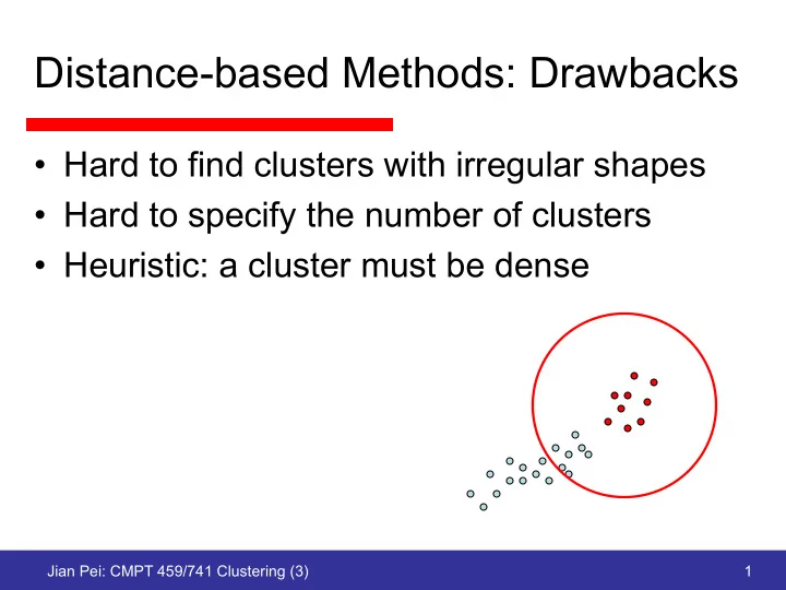
- Hard to find clusters with irregular shapes
- Hard to specify the number of clusters
- Heuristic: a cluster must be dense