[PPT] - Discrete time Markov chains Today: Random walks First step PowerPoint Presentation

SLIDE 1

Random walks and branching processess

Bo Friis Nielsen1

1DTU Informatics

02407 Stochastic Processes 2, September 6 2016

Bo Friis Nielsen Random walks and branching processess

Discrete time Markov chains

Today:

◮ Random walks ◮ First step analysis revisited ◮ Branching processes ◮ Generating functions

Next week

◮ Classification of states ◮ Classification of chains ◮ Discrete time Markov chains - invariant probability

distribution Two weeks from now

◮ Poisson process

Bo Friis Nielsen Random walks and branching processess

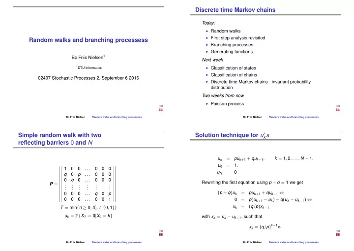
Simple random walk with two reflecting barriers 0 and N

P =

1

. . . q p . . . q . . . . . . . . . . . . . . . . . . . . . . . . . . . q p . . . 1

T = min{n ≥ 0; Xn ∈ {0, 1}}

uk = P{XT = 0|X0 = k}

Bo Friis Nielsen Random walks and branching processess

Solution technique for u′

ks

uk = puk+1 + quk−1, k = 1, 2, . . . , N − 1, u0 = 1, uN = Rewriting the first equation using p + q = 1 we get (p + q)uk = puk+1 + quk−1 ⇔ = p(uk+1 − uk) − q(uk − uk−1) ⇔ xk = (q/p)xk−1 with xk = uk − uk−1, such that xk = (q/p)k−1x1

Bo Friis Nielsen Random walks and branching processess

SLIDE 2

Recovering uk

x1 = u1 − u0 = u1 − 1 x2 = u2 − u1 . . . xk = uk − uk−1 such that u1 = x1 + 1 u2 = x2 + x1 + 1 . . . uk = xk + xk−1 + · · · + 1 = 1 + x1

k−1

i=0

(q/p)i

Bo Friis Nielsen Random walks and branching processess

Values of absorption probabilities uk

From uN = 0 we get = 1 + x1

N−1

i=0

(q/p)i ⇔ x1 = − 1 N−1

i=0 (q/p)i

Leading to uk =

1 − (k/N) = (N − k)/N

when p = q = 1

2 (q/p)k−(q/p)N 1−(q/p)N

when p = q

Bo Friis Nielsen Random walks and branching processess

Direct calculation as opposed to first step analysis

P =

Q

R I

P2

=

Q

R I

Q

R I

=
Q2

QR + R I

Pn

=

Qn

Qn−1R + Qn−2R + · · · + QR + R I

W (n)

ij

= E n

ℓ=0

1(Xℓ = j)|X0 = i

, where 1(Xℓ) =

1 if Xℓ = j if Xℓ = j

Bo Friis Nielsen Random walks and branching processess

Expected number of visits to states

W (n)

ij

= Q(0)

ij

+ Q(1)

ij

+ . . . Q(n)

ij

In matrix notation we get W (n) = I + Q + Q2 + · · · + Qn = I + Q

I + Q + · · · + Qn−1

= I + QW (n−1) Elementwise we get the “first step analysis” equations W (n)

ij

= δij +

r−1

k=0

PikW (n−1)

kj

Bo Friis Nielsen Random walks and branching processess

SLIDE 3

Limiting equations as n → ∞

W = I + Q + Q2 + · · · =

∞

i=0

Qi W = I + QW From the latter we get (I − Q)W = I When all states related to Q are transient (we have assumed that) we have W =

∞

i=0

Qi = (I − Q)−1 With T = min{n ≥ 0, r ≤ Xn ≤ N} we have that Wij = E T−1

n=0

1(Xn = j)

X0 = i
Bo Friis Nielsen

Random walks and branching processess

Absorption time

T−1

n=0

r

j=0

1(Xn = j) =

T−1

n=0

1 = T Thus E(T|X0 = i) = E  

r

j=0

T−1

n=0

1(Xn = j) X0 = i   =

r

j=0

E T−1

n=0

1(Xn = j|X0 = i

=

r

j=0

Wij In matrix formulation v = W1 where vi = E(T|X0 = i) as last week, and 1 is a column vector

f ones.

Bo Friis Nielsen Random walks and branching processess

Absorption probabilities

U(n)

ij

= P{T ≤ n, XT = j|X0 = i} U(1) = R = IR U(2) = IR + QR U(n) = (I + Q + · · · + Q(n−1)R = W (n−1)R Leading to U = WR

Bo Friis Nielsen Random walks and branching processess

Random sum (2.3)

X = ξ1 + · · · + ξN =

N

i=1

ξi where N is a random variable taking values among the non-negative integers; with E(N) = ν, Var(N) = τ 2, E(ξi) = µ, Var(ξi) = σ2 E(X) = E(E(X|N)) = E(Nµ) = νµ Var(X) = E(Var(X|N)) + Var(E(X|N)) = E(Nσ2) + Var(Nµ) = νσ2 + τ 2µ2

Bo Friis Nielsen Random walks and branching processess

SLIDE 4

Branching processes

Xn+1 = ξ1 + ξ2 + · · · + ξXn where ξi are independent random variables with common propability mass function P{ξi = k} = pk From a random sum interpretation we get E(Xn+1) = µE(Xn) = µn+1 Var(Xn+1) = σ2E(Xn) + µVar(Xn) = σ2µn + µ2Var(Xn) = σ2µn + µ2(σ2µn−1 + µ2Var(Xn−1))

Bo Friis Nielsen Random walks and branching processess

Extinction probabilities

Define N to be the random time of extinction (N can be defective - i.e. P{N = ∞) > 0)} un = P{N ≤ n} = P{XN = 0} And we get un =

∞

k=0

pkuk

n−1

Bo Friis Nielsen Random walks and branching processess

The generating function - an important analytic tool

◮ Manipulations with probability distributions ◮ Determining the distribution of a sum of random variables ◮ Determining the distribution of a random sum of random

variables

◮ Calculation of moments ◮ Unique characterisation of the distribution ◮ Same information as CDF

Bo Friis Nielsen Random walks and branching processess

Generating functions

φ(s) = E

sξ

=

∞

k=0

pksk, pk = 1 k! dkφ(s) dsk

s=0

Moments from generating functions dφ(s) ds

s=1

=

∞

k=1

pkksk−1

s=1

= E(ξ) Similarly d2φ(s) ds2

s=1

=

∞

k=2

pkk(k − 1)sk−2

s=1

= E(ξ(ξ − 1)) a factorial moment Var(ξ) = φ′′(1) + φ′(1) − (φ′(1))2

Bo Friis Nielsen Random walks and branching processess

SLIDE 5

The sum of iid random variables

Remember Independent Identically Distributed Sn = X1 + X2 + · · · + Xn = n

i=1 Xi

With px = P{Xi = x}, Xi ≥ 0 we find for n = 2 S2 = X1 + X2 The event {S2 = x} can be decomposed into the set {(X1 = 0, X2 = x), (X1 = 1, X2 = x − 1) . . . (X1 = i, X2 = x − i), . . . (X1 = x, X2 = 0)} The probability of the event {S2 = x} is the sum of the probabilities of the individual outcomes.

Bo Friis Nielsen Random walks and branching processess

Sum of iid random variables - continued

The Probability of outcome (X1 = i, X2 = x − i) is P{X1 = i, X2 = x − i} = P{X1 = i}P{X2 = x − i} by independence, which again is pipx−i. In total we get P{S2 = x} =

x

i=0

pipx−i

Bo Friis Nielsen Random walks and branching processess

Generating function - one example

Binomial distribution pk = n k

pk(1 − p)n−k

φbin(s) =

n

k=0

skpk =

n

k=0

sk n k

pk(1 − p)n−k

=

n

k=0

n k

(sp)k(1 − p)n−k = (1 − p + ps)n

Bo Friis Nielsen Random walks and branching processess

Generating function - another example

Poisson distribution pk = λk k! e−λ φpoi(s) =

∞

k=0

skpk =

∞

k=0

sk λk k! e−λ = e−λ

∞

k=0

(sλ)k k! = e−λesλ = e−λ(1−s)

Bo Friis Nielsen Random walks and branching processess

SLIDE 6

And now to the reason for all this . . .

The convolution can be tough to deal with (sum of random variables) Theorem If X and Y are independent then φX+Y(s) = φX(s)φY(s) where φX(s) and φY(s) are the generating functions of X and Y

A probabilistic proof (which I think is instructive)

φX+Y(s) = E

sX+Y

= E

sXsY

= E

sX

E

sY

= φX(s)φY(s)

Bo Friis Nielsen Random walks and branching processess

Sum of two Poisson distributed random variables

X ∼ P(λ) Y ∼ P(µ) Z = X + Y φX(s) = e−λ(1−s) φY(s) = e−µ(1−s)

P{X = x} = px = λx

x! e−λ

And we get

φZ(s) = φX(s)φY(s) = e−λ(1−s)e−µ(1−s) = e−(λ+µ)(1−s) Such that Z ∼ P(λ + µ)

Bo Friis Nielsen Random walks and branching processess

Sum of two Binomial random variables with the same p

X ∼ B(n, p) Y ∼ B(m, p) Z = X + Y φX(s) = (1 − p + ps)n φY(s) = (1 − p + ps)m

P{X = x} = px =

n x

px(1 − p)n−x
And we get

φZ(s) = φX(s)φY(s) = (1−p+ps)n(1−p+ps)m = (1−p+ps)n+m Such that Z ∼ B(n + m, p)

Bo Friis Nielsen Random walks and branching processess

Poisson example

X ∼ P(λ) φX(s) = e−λ(1−s)

P{X = x} = px = λx

x! e−λ

φ′(s) = −(−λ)e−λ(1−s) = λe−λ(1−s)

And we find E(X) = φ′(1) = λe0 = λ φ′′(s) = λ2e−λ(1−s) V(X) = φ′′(1) + φ′(1) − (φ′(1))2 = λ2 + λ − λ2 = λ

Bo Friis Nielsen Random walks and branching processess

SLIDE 7

Generating function - the geometric distribution

px = (1 − p)x−1p φgeo(s) =

∞

x=1

sxpx =

∞

x=1

sx(1 − p)x−1p =

∞

x=1

s(s(1 − p))x−1p A useful power series is:

N

i=0

ai =     

1−aN+1 1−a

N < ∞, a = 1 N + 1 N < ∞, a = 1

1 1−a

N = ∞, |a| < 1 And we get φgeo(s) = sp 1 − s(1 − p)

Bo Friis Nielsen Random walks and branching processess

Generating function for random sum

hX(s) = gN(φ(s)) Applied for the branching process we get φn(s) = φn−1(φ(s))

Bo Friis Nielsen Random walks and branching processess

Generating function for the sum of independent random variables

X with pdf px Y with pdf qy Z = X + Y what is rz = P{Z = z}? P{Z = z} = rz =

z

i=0

piqz−i Theorem (23) page 153 If X and Y are independent then φX+Y(s) = φX(s)φY(s) where φX(s) and φY(s) are the generating functions of X and Y

Bo Friis Nielsen

Random walks and branching processess

Sum of two geometric random variables with the same p

X ∼ geo(p) Y ∼ geo(p) Z = X + Y φX(s) =

sp 1−s(1−p)

φY(s) =

sp 1−s(1−p)

P{X = x} = px = (1 − p)x−1p
And we get

φZ(s) = φX(s)φY(s) = sp 1 − s(1 − p) sp 1 − s(1 − p) =

sp

(1 − s(1 − p) 2 The density of this distribution is P{Z = z} = h(z) = (z − 1)(1 − p)z−2p2 Negative binomial.

Bo Friis Nielsen Random walks and branching processess

SLIDE 8

Sum of k geometric random variables with the same p

More generally - sum of k geometric variables px = x − 1 k − 1

(1 − p)x−kpk

φX(s) =

sp

1 − s(1 − p) k

Bo Friis Nielsen Random walks and branching processess

Characteristic function and other

◮ Characteristic function: E

eitX

◮ Moment generating function: E

eθX

◮ Laplace Stieltjes transform: E

e−sX

EXAMPLE: (exponential) E

eθX

= ∞ eθxλe−λxdx = λ λ − θ, θ < λ

Bo Friis Nielsen Random walks and branching processess