
SLIDE 1 Review
- f
- V
- ints H
- S op
- f
HYPOTHESIS SET ALGORITHM LEARNING FINAL HYPOTHESIS H A
g ~ f ~ f: X Y
TRAINING EXAMPLES UNKNOWN TARGET FUNCTION DISTRIBUTION PROBABILITY
- n
P
X
x y x y
N N 1 1
( , ), ... , ( , )
up down
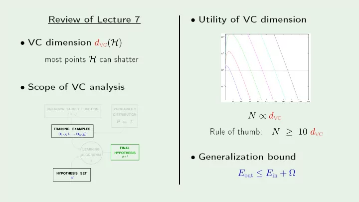
- Utilit
- f
20 40 60 80 100 120 140 160 180 200 10
−5
10 10
5
10
10
N ∝ d
v Rule- f
N ≥ 10 d
v- Generalization
- und
E
- ut ≤ E