Determining Location from Pop up Satellite Archival Transmitters - - PowerPoint PPT Presentation

determining location from pop up satellite archival
SMART_READER_LITE
LIVE PREVIEW

Determining Location from Pop up Satellite Archival Transmitters - - PowerPoint PPT Presentation

Determining Location from Pop up Satellite Archival Transmitters (PSATs) When Earth Main Field Geomagnetic Data Is Insufficient: A Case Study with Lake Sturgeon in Eastern Lake Erie Davis, Lori 1* , R. Neuenhoff 1 , J.L. Withers 1 , J.A. Sweka 1


slide-1
SLIDE 1

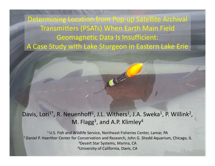
Determining Location from Pop‐up Satellite Archival Transmitters (PSATs) When Earth Main Field Geomagnetic Data Is Insufficient: A Case Study with Lake Sturgeon in Eastern Lake Erie

Davis, Lori1*, R. Neuenhoff1, J.L. Withers1, J.A. Sweka1, P. Willink2,

  • M. Flagg3, and A.P. Klimley4

1 U.S. Fish and Wildlife Service, Northeast Fisheries Center, Lamar, PA 2 Daniel P. Haerther Center for Conservation and Research, John G. Shedd Aquarium, Chicago, IL 3Desert Star Systems, Marina, CA 4University of California, Davis, CA

slide-2
SLIDE 2

Objectives

  • Characterize

movement and habitat use of adult Lake Sturgeon in Buffalo Harbor, Lake Erie

slide-3
SLIDE 3

Study Area

slide-4
SLIDE 4

Study Area

Source: Esri, DigitalGlobe, GeoEye, Earthstar Geographics, CNES/Airbus DS, USDA, USGS, AEX, Getmapping, Aerogrid, IGN, IGP, swisstopo, and the GIS User Community

Ü

30 60 90 120 15 Kilometers

slide-5
SLIDE 5

Equipment

  • SeaMOD‐tag (PSATs) product of Desert Star

Systems

– Sampling interval: 4 minutes – Measurements: depth (m), temperature (C), day length, 3 axis acceleration, 3 axis magnetic field, etc.

slide-6
SLIDE 6

PSATs deployed

  • Year 1 (2014) – 23

– 7 = 3‐5 months – 16 = 12 months

  • Year 2 (2015) – 9

– 4 = 5 month – 5 = 12 month

  • Year 3 (2016) – 10

– 10 = 14 months

slide-7
SLIDE 7

Year 1 Deployment

  • Challenges Encountered

– Constant depth release (CDR)

  • Trigger release if observed constant depth for “x” days
  • Bathymetry of area

‐2 2 4 6 8 10 12 Depth (m)

Depth (m)

5/29/2014 6/11/2014

CDR

slide-8
SLIDE 8

Year 1 Challenges cont.

– Attachment method led to shed/thrown PSATs

  • Two single points
slide-9
SLIDE 9

Year 2 Deployment

  • Address challenges encountered in Year 1

– Turned off Constant Depth Release – Moved to double point of attachment method

  • Lacroix
slide-10
SLIDE 10
slide-11
SLIDE 11

Year 2 Deployment

  • Challenges Encountered – Argos Data

– Very few priority or sensor data packets – Made locating PSATs for recovery and download difficult

Year Total Transmissions Transmissions Quality 3 or 2 Year 1‐ 2014 33243 8496 Year 2‐ 2015 58 4

slide-12
SLIDE 12

Solution?

slide-13
SLIDE 13

1 of 9 RECOVERED in 2015!

slide-14
SLIDE 14

Year 2 Challenges Cont.

  • Daily positional information outputted by

SeaTrack software not accurate

slide-15
SLIDE 15

SeaTrack Output

slide-16
SLIDE 16

Year 2 Challenges Cont.

  • Seatrack Software

– Day length: Longitude (East‐West) – Total Magnetic Field (nT): Latitude (North‐South) Day Length + Magnetic Field = Location

slide-17
SLIDE 17
slide-18
SLIDE 18

Earth Main Geomagnetic Field (nT)

Lake Erie

Magnetic Field (nT) =Traveling North

slide-19
SLIDE 19

Archived Data – Recovered PSAT

53000 53200 53400 53600 53800 54000 54200 54400 Magnetic Field (nT) Magnetic Field Intensity (nT) Approx Magnetic Field Intensity (nT)

slide-20
SLIDE 20

SeaTrack Output

slide-21
SLIDE 21

Year 2 Challenges Cont.

  • Daily positional information outputted by

SeaTrack software not accurate enough

  • Earth main geomagnetic field may be

insufficient for determining position

– PSAT magnetic field readings may potentially heavily influenced by variations in the magnetic field occurring at the local level

slide-22
SLIDE 22

Unique Opportunity

  • Lake Sturgeon dual tagged

with Vemco V16 acoustic transmitter and PSAT

slide-23
SLIDE 23

Applying other methods….

  • Methods developed by Flagg et al.

– Use other data collected and archived by PSAT to determine position

  • Depth
  • Accelerometer
  • Calculated magnetic anomaly
  • Temperature

– Temporally heterogeneous but spatially homogeneous

slide-24
SLIDE 24

July 7/05/2015‐ 7/31/2015

5 10 15 20 25 30 35 40 45 50 0.00 2.00 4.00 6.00 8.00 10.00 12.00 14.00 16.00 6/30/15 0:00 7/5/15 0:00 7/10/15 0:00 7/15/15 0:00 7/20/15 0:00 7/25/15 0:00 7/30/15 0:00 8/4/15 0:00

Depth (ft) Depth (m) Date

slide-25
SLIDE 25

July 7/15/2015‐ 7/17/2015

0.2 0.4 0.6 0.8 1 1.2 Acceleration (G)

Acceleration Z‐axis

acceleration Z‐ axis (G) Hourly avg acceleration Z‐ axis (G)

Z‐Axis 1G <1G

slide-26
SLIDE 26

Applying other methods… Magnetic data

Legend

+250 nT +150 nT 0 nT ‐100 nT ‐200 nT ‐300 nT

Data source: Geological Survey Canada

slide-27
SLIDE 27

Challenges still…

  • Able to draw conclusions on movement based on

depth but relayed heavily on acoustic information

  • Local anomalies in the magnetic field may still exist

at ground/sea level

– Some effort associated with this type of survey – What degree of variation exist?

  • Error of +/‐ 100nT
  • Temperature

– Not a uniform bias

slide-28
SLIDE 28

Acknowledgements

  • Great Lakes Restoration Initiative (GLRI)
  • Great Lakes Acoustic Telemetry Observation

System (GLATOS)

  • Buffalo State University of New York
  • Michigan Department of Natural Resources
  • New York State Department of

Environmental Conservation

  • Ohio Department of Natural Resources
  • Ontario Ministry of Natural Resources
  • Pennsylvania Fish and Boat Commission
  • Shedd Aquarium
  • U.S. Army Corps of Engineers
  • U.S. Coast Guard
  • U.S. Fish and Wildlife Service, Alpena Fish

and Wildlife Conservation Office

  • U.S. Fish and Wildlife Service, Lower Great

Lakes Fish and Wildlife Conservation Office

slide-29
SLIDE 29

Questions?