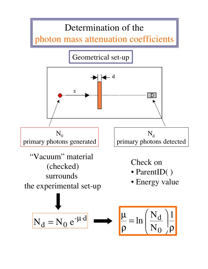
Determination of the photon mass attenuation coefficients - PDF document

Determination of the photon mass attenuation coefficients Geometrical set-up N 0 N d primary photons generated primary photons detected “Vacuum” material Check on (checked) • ParentID( ) surrounds • Energy value the experimental set-up   µ N 1 µ ⋅ =   d - d = ln   N N e ρ ρ d 0   N 0

E.M processes implemented • E.M. Standard •G4PhotoElectricEffect •G4ComptonScattering •G4GammaConversion • Low Energy •G4LowEnergyRayleigh •G4LowEnergyPhotoElectric •G4LowEnergyCompton •G4LowEnergyGammaConversion Simulation in water, iron, lead with E.M.Standard and LowE extension and comparison with the National Institute for Standard and Technology (NIST) data

Photon mass attenuation coefficient, Water LowE E.M. Standard Geant4 EMStandard Geant4 LowEn 10 10 NIST NIST µ / ρ (cm 2 / g) in water µ / ρ (cm 2 /g) in water 1 1 0.1 0.1 0.01 0.1 1 10 0.01 0.1 1 10 Photon Energy (MeV) Photon Energy (MeV) Differences % Delta = (NIST-G4EMStand) / NIST Delta = (NIST-G4LowEn) / NIST 16 14 12 10 8 6 4 2 Delta (%) 0 -2 -4 -6 -8 -10 -12 -14 -16 0.01 0.1 1 10 Photon Energy (MeV)

Photon mass attenuation coefficient, Iron LowE E.M. Standard Geant4 LowEn 1000 Geant4 EMStandard 1000 NIST NIST 2 /g) in iron 100 µ / ρ (cm 2 / g) in iron 100 10 10 µ / ρ (cm 1 1 0.1 0.1 0.01 0.01 0.01 0.1 1 10 0.01 0.1 1 10 Photon Energy (MeV) Photon Energy (MeV) Differences % E = (NIST-G4EMStandard)/NIST 18 E = (NIST-G4LowEn)/NIST 16 14 12 10 8 6 4 2 E (%) 0 -2 -4 -6 -8 -10 -12 -14 -16 -18 0.01 0.1 1 10 Photon Energy (MeV)

Photon mass attenuation coefficient, Lead LowE E.M. Standard Geant4 LowEn NIST Geant4 EMStandard NIST 100 100 µ / ρ (cm 2 / g in lead 10 µ / ρ (cm 2 / g in lead 10 1 1 0.1 0.1 0.01 0.01 0.01 0.1 1 0.01 0.1 1 Photon energy (MeV) Photon energy (MeV) Below 100 KeV zero photons are detected, all the photons have interaction Differences % E = (NIST - G4EM Standard)/NIST 10 E = (NIST- G4LowEn)/NIST 8 6 4 2 E (%) 0 -2 -4 -6 -8 -10 0.01 0.1 1 Photon Energy (MeV)

Determination of the isodose distribution in water around a 192 Ir source The microSelectron HDR 192 Ir source 192 Ir Photon (gamma + x ray) spectrum of Iridium is complex: ~ 24 lines in the energy range 9 -885 KeV Our Primary Generator (simplified monochromatic model) G4ParticleGun shoots gamma • random position inside the iridium core • random direction • mean energy <E> = 356 KeV Stainless steel capsule and cable

Geometrical set-up The source is placed inside a 30 cm water box which is associated with a Sensitive Detector object We wish to determine the energy deposition in water around the source in a longitudinal plane (cylindrical symmetry) Readout Geometry The longitudinal plane is portioned in 300 · 300, 1 mm 3 , voxels 192 Ir At every interaction, energy deposition is scored and stored in the relevant voxel (in a matrix)

EM Processes implemented • G4MultipleScattering gamma • G4LowEnergyRayleigh • G4LowEnergyPhotoElectric • G4LowEnergyCompton • G4LowEnergyGammaConversion e- • G4LowEnergyIonisation • G4LowEnergyBremsstrahlung e+ • G4eIonisation • G4eBremsstrahlung • G4eplusAnnihilation Output As in the advanced Brachytherapy example, at the end of the RUN an ASCII file is produced for further processing with X,Z energy deposition

Isodose distribution in water around a 192 Ir source • 20 10 6 photons generated • ~ 24 hours of simulation 40 Isodose Distance along longitudinal axis (mm) 30 200% 150% 20 100% 10 75% 50% 0 25% -10 -20 -30 -40 -40 -30 -20 -10 0 10 20 30 40 Distance along transverse axis (mm) The dose deposition is not isotropic due to •source geometry •auto-absorption, •encapsulation and shielding effects At the bottom centre of the source we can see the effect of the stainless steel cable

Comparison with isodoses of the Plato treatment planning system 40 Isodose Distance along longitudinal axis (mm) 30 200% 150% 20 100% 10 75% 50% 0 25% -10 -20 -30 -40 -40 -30 -20 -10 0 10 20 30 40 Distance along transverse axis (mm) 1 cm Plato uses an analytical method to calculate the dose distribution: • Point approximation of the source to compute the dose • Anisotropy function F( ϕ ), instead of F(r, ϕ ) as it should be, to account for the shielding effect of the capsule, etc..

Comparison with the isodoses of the Plato treatment planning system Transverse axis 3.0 Our simulation Plato 2.5 2.0 PDD (%) • Good agreement 1.5 1.0 0.5 0.0 0 10 20 30 40 50 Distance along transverse axis (mm) Longitudinal axis Our simulation Plato 3.0 2.5 2.0 • Good agreement PDD(%) 1.5 in front of the source 1.0 • Less good agreement 0.5 behind the source 0.0 -50 -40 -30 -20 -10 0 10 20 30 40 50 Distance along longitudinal axis (mm) The disagreement in the region behind the source is due to the approximation introduced by the anisotropy function in this direction Geant4 yields a more realistic behaviour

Initial results for the Leipzig applicator The Leipzig applicators were designed to give the optimum isodoses and treat to the correct depth This applicator has the shape of a hollow cylinder of tungsten containing the source Geometrical set-up Iridium source Applicator Water box & ROGeometry

Isodose distribution in water for the Leipzig applicator Distance (mm) -40 -20 0 20 40 0 isodose -10 80% Depth from surface (mm) 60% 40% -20 20% 10% -30 -40 -50 • 10 8 photons generated • ~ 4 days of CPU Our simulation time Nucletron Data 0.8 Our measurements 0.6 Preliminary PDD (%) 0.4 0.2 0.0 0 10 20 30 40 50 Depth from surface (mm) These are the initial results with this kind of applicator • good agreement with manufacturer’s data (Nucletron) • satisfactory agreement with our measurements (we have just started making measurements and the systematic errors for the response of the detector are not well known yet)

Conclusion Our activities at · Porting on Windows 98+Cygwin+VisualC++ environment · Simple test for the EM processes · Application in the medical field Simulation for isodose distribution and comparison of the result with those of our TPS and measure · Promotion of Geant4 with poster and oral presentation in several medical physics congress (AIFM, ESTRO, AIRO, …) We think that Geant4 is an useful instrument in medical radiation physics Its use out of the HEP community could be advantageous both for users (as we are) and for the code developers