det ( I + zK ) = i , j = 1 K ( t i , t j ) dt det ( m) (d) n ! - - PowerPoint PPT Presentation

ZENTRUM MATHEMATIK TECHNISCHE UNIVERSITÄT MÜNCHEN

Very Special Functions — unbeknownst to Mathematica and kinship numerical explorations of random matrix distributions

(a) (c)

• 1000
• 500

500 1000

• 1000
• 500

500 1000 1000 2000 3000 500 1000 1500 2000

(b) (d)

(µm) (µm)

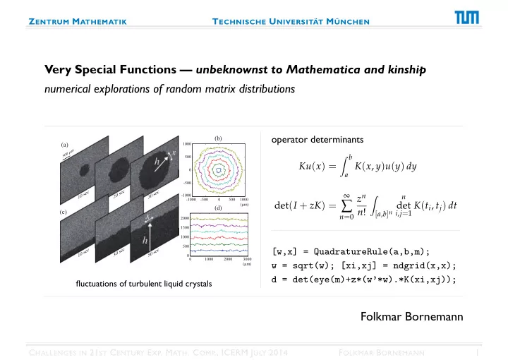
fluctuations of turbulent liquid crystals

• perator determinants

Ku(x) =

b

a K(x, y)u(y) dy

det(I + zK) =

∞

∑

n=0

zn n!

• [a,b]n

n

det

i,j=1 K(ti, tj) dt

[w,x] = QuadratureRule(a,b,m); w = sqrt(w); [xi,xj] = ndgrid(x,x); d = det(eye(m)+z*(w’*w).*K(xi,xj));

Folkmar Bornemann

CHALLENGES IN 21ST CENTURY EXP. MATH. COMP., ICERM JULY 2014 FOLKMAR BORNEMANN 1

SCALING LIMITS OF RANDOM MATRICES

example: GUE

Gaussian unitary ensemble

A = randn(n) + i*randn(n); A = (A+A’)/2;

spectrum as n → ∞? fluctuations?

Wigner semicircle law (1955)

probability density eigenvalues/√n −2 −1 1 2 0.1 0.2 0.3 0.4 0.5

bulk: Gaudin–Mehta distribution E2

probability density normalized eigenvalue spacing 0.5 1 1.5 2 2.5 3 0.2 0.4 0.6 0.8 1

edge: Tracy–Widom distribution F2

probability density normalized maximum eigenvalue −5 −4 −3 −2 −1 1 2 0.1 0.2 0.3 0.4 0.5

universality: fluctuation statistics does only depend on symmetry class (Soshnikov; Tao; L. Erd˝

• s, . . . )

CHALLENGES IN 21ST CENTURY EXP. MATH. COMP., ICERM JULY 2014 FOLKMAR BORNEMANN 2

UNIVERSALITY WITHIN MATHEMATICS

Montgomery–Odlzyko “law” (’73/’87) nontrivial zeros 1

2 + iγn of Riemann ζ-function

large n statistics of the spacings of γn 2π log γn 2π

→ Gaudin–Mehta distribution E2

0.5 1 1.5 2 2.5 3 0.1 0.2 0.3 0.4 0.5 0.6 0.7 0.8 0.9 1

Normalized consecutive spacings Probability density

Montgomery−Odlyzko law

fluctuations in Ulam’s problem (Baik/Deift/Johansson ’99) ln = length of longest increasing subsequence of a random permutation of order n ln − 2√n n1/6

→ Tracy–Widom distribution F2

CHALLENGES IN 21ST CENTURY EXP. MATH. COMP., ICERM JULY 2014 FOLKMAR BORNEMANN 3

UNIVERSALITY: A VERY SHORT INTRODUCTION

• H. Spohn: Random Matrices and the KPZ Equation (June 1, ’12, HCM, Bonn)

Universality: The macroscopic statistics depend on the models, but the microscopic statistics are independent of the details of the systems except the symmetries. — L. Erd˝

• s ’10

CHALLENGES IN 21ST CENTURY EXP. MATH. COMP., ICERM JULY 2014 FOLKMAR BORNEMANN 4

B./Ferrari/Prähofer '08

VERY SPECIAL FUNCTIONS, INDEED

spacing distributions of GUE @ bulk P(exactly n eigenvalues in (0, s)) = (−1)n n! ∂n ∂zn E2(s; z)

• z=1

Gaudin ’61

E2(s; z) = det

• I − zK|L2(0,s)
• w/ kernel

K(x, y) = sinc(π(x − y)) can be expressed in terms of radial prolate spheroidal wave functions

Jimbo/Miwa/Môri/Sato ’80

E2(s; z) = exp

• −

πs

σ(x; z) x dx

• w/ σ-form of Painlevé V

(xσ′′)2 = 4(σ − xσ′)(xσ′ − σ − σ′ 2)

σ(x; z) ≃ z π x + z2 π2 x2

(x → 0)

CHALLENGES IN 21ST CENTURY EXP. MATH. COMP., ICERM JULY 2014 FOLKMAR BORNEMANN 5

VERY SPECIAL FUNCTIONS, VERY MUCH SO INDEED

spacing distributions of GUE @ soft edge P(exactly n eigenvalues in (s, ∞)) = (−1)n n! ∂n ∂zn F2(s; z)

• z=1

Forrester ’93

F2(s; z) = det

• I − z K|L2(s,∞)
• w/ kernel

K(x, y) = Ai(x) Ai′(y) − Ai′(x) Ai(y) x − y

Tracy/Widom ’93

F2(s; z) = exp

• −

∞

s (x − s)u(x; z)2 dx

• w/ Painlevé II

u′′ = 2u3 + xu u(x; z) ≃ √ z Ai(x)

(x → ∞)

Without the Painlevé representations, the numerical evaluation of the Fredholm determinants is quite involved. — Tracy/Widom ’00 Recently a numerical analyst has shown that the most efficient way to compute spacing distributions in classical RMT is to use Fredholm determinant formulas. — Forrester ’10

CHALLENGES IN 21ST CENTURY EXP. MATH. COMP., ICERM JULY 2014 FOLKMAR BORNEMANN 6

FREDHOLM DETERMINANTS VS. PAINLEVÉ TRANSCENDENTS

very special functions: nonlinear ode, but integrable

Ivar Fredholm (1866–1927)

determinant of integral operator (1899) Ku(x) =

b

a K(x, y)u(y) dy

• det(I + zK) =

∞

∑

n=0

zn n!

• [a,b]n

n

det

i,j=1 K(ti, tj) dt

Paul Painlevé (1863–1933)

six families of irreducible transcendental functions (1895) u′′ = 6u2 + x u′′ = 2u3 + xu − α u′′ = u−1u′ 2 − x−1u′ + x−1(αu2 + β) + γu3 + δu−1 . . .

CHALLENGES IN 21ST CENTURY EXP. MATH. COMP., ICERM JULY 2014 FOLKMAR BORNEMANN 7

COMPARING DIFFERENT NUMERICAL APPROACHES

numerical evaluation of the Tracy–Widom distribution F2

−8 −6 −4 −2 2 4 6 8 10

−20

10

−15

10

−10

10

−5

10

x absolute error

Painlevé II by IVP F2(x) by IVP Painlevé II by BVP F2(x) by BVP F2(x) by Fredholm machine precision

absolute error using IEEE double precision

• via Painlevé II as IVP (backwards)

Prähofer (’04): 16 digits (1500 internally!) Bejan (’05): 3 digits Edelman/Persson (’05): 8 digits @ 8.9 sec

• via Painlevé II as BVP

Tracy/Widom (’94): 10 digits (75 internally!) Dieng (’05): 9 digits @ 3.7 sec Driscoll/B./Trefethen (’08): 13 digits @ 1.3 sec

• via Fredholm determinant
• B. (’10): 15 digits @ 0.69 sec

CHALLENGES IN 21ST CENTURY EXP. MATH. COMP., ICERM JULY 2014 FOLKMAR BORNEMANN 8

THE NEED FOR CONNECTION FORMULAE

instability solution of Painlevé II, uxx = 2u3 + xu, u(x) ≃ √ z Ai(x)

(x → ∞),

separatrix for z = 1

IVP highly unstable

14 12 10 8 6 4 2 2 4

x

2 2 4

ux

u(x) with √z = 1 − 10−8, 1, 1 + 10−8

14 12 10 8 6 4 2 2 4

x

2 2 4

ux

u(x) with √z = 1 − 10−16, 1, 1 + 10−16

consequence

• calculate F2 via a BVP solution connection formula needed:

u(x) ≃ √ z Ai(x)

(x → ∞) ⇒

u(x) ≃ ?

(x → −∞)

CHALLENGES IN 21ST CENTURY EXP. MATH. COMP., ICERM JULY 2014 FOLKMAR BORNEMANN 9

THE NEED FOR CONNECTION FORMULAE

instability solution of Painlevé II, uxx = 2u3 + xu, u(x) ≃ √ z Ai(x)

(x → ∞),

separatrix for z = 1

IVP highly unstable

14 12 10 8 6 4 2 2 4

x

2 2 4

ux

u(x) with √z = 1 − 10−8, 1, 1 + 10−8

14 12 10 8 6 4 2 2 4

x

2 2 4

ux

u(x) with √z = 1 − 10−16, 1, 1 + 10−16

consequence

• calculate F2 via a BVP solution connection formula needed:

u(x) ≃ Ai(x)

(x → ∞) ⇒

u(x) ≃

√ −x/2 (x → −∞)

CHALLENGES IN 21ST CENTURY EXP. MATH. COMP., ICERM JULY 2014 FOLKMAR BORNEMANN 9

QUADRATURE METHOD

Nyström (1930) solved a Fredholm equation (I + zK)u = f of the 2nd kind, u(x) + z

b

a K(x, y)u(y) dy = f (x)

(x ∈ (a, b)),

using an m-point quadrature formula w/ weights wj & nodes xj

Evert Nyström (1895–1960)

u(xi) ≈ ui : ui + z

m

∑

j=1

wjK(xi, xj)uj = f (xi)

(i = 1, . . . , m)

straightforward idea (B. ’08) approximate det(I + zK) simply by the corresponding n × n determinant det

• I + z (wjK(xi, xj))m

i,j=1

• CHALLENGES IN 21ST CENTURY EXP. MATH. COMP., ICERM JULY 2014

FOLKMAR BORNEMANN 10

CONVERGENCE RATE OF THE QUADRATURE METHOD

Matlab code [w,x] = QuadratureRule(a,b,m); w = sqrt(w); [xi,xj] = ndgrid(x,x); d = det(eye(m)+z*(w’*w).*K(xi,xj)); Theorem (B. ’10) for quadrature formula of order ν w/ positive weights:

• if kernel is Ck−1,1([a, b]2),

error = O(ν−k);

• if kernel is bounded analytic, there is ρ > 1 w/

error = O(ρ−ν).

CHALLENGES IN 21ST CENTURY EXP. MATH. COMP., ICERM JULY 2014 FOLKMAR BORNEMANN 11

PROOF

idea of proof (Hilbert 1904, B. ’10) m-point quadrature formula

b

a f (t) dt ≈ m

∑

k=1

wk f (xk) yields det(I + zK)

Fredholm

=

1903

∞

∑

n=0

zn n!

b

a

dt1 · · ·

b

a

dtn

n

det

i,j=1 K(ti, tj)

Hadamard

≈

1893

∞

∑

n=0

zn n!

m

∑

k1=1

wk1 · · ·

m

∑

kn=1

wkn

n

det

i,j=1 K(xki, xkj)

• v. Koch

=

1892

det(I + zKm) w/ the m × m-matrix Km =

• w1/2

i

K(xi, xj)w1/2

j

m

i,j=1

CHALLENGES IN 21ST CENTURY EXP. MATH. COMP., ICERM JULY 2014 FOLKMAR BORNEMANN 12

EXAMPLE 1

Gaudin–Mehta distribution E2 E2(0; s) = det

• I − K|L2(0,s)
• ,

K(x, y) = sinc(π(x − y))

5 10 15 20 25 10

−20

10

−15

10

−10

10

−5

10

dimension approximation error for E2(0;2)

stars: Gaudin’s method, dots: Gauss–Legendre, circles: Clenshaw–Curtis CHALLENGES IN 21ST CENTURY EXP. MATH. COMP., ICERM JULY 2014 FOLKMAR BORNEMANN 13

EXAMPLE 2

Tracy–Widom distribution F2 F2(s) = det

• I − K|L2(s,∞)
• ,

K(x, y) = Ai(x) Ai′(y) − Ai′(x) Ai(y) x − y

5 10 15 20 25 30 35 40 45 50 10

−20

10

−15

10

−10

10

−5

10

dimension approximation error for F2(−2)

dots: Gauss–Legendre, circles: Clenshaw–Curtis

perturbation bound for m-dimensional determinants: (B. ’10) round-off error √ m KmF · ǫmachine

CHALLENGES IN 21ST CENTURY EXP. MATH. COMP., ICERM JULY 2014 FOLKMAR BORNEMANN 14

DYSON BROWNIAN MOTION

An(t) n × n hermitean-matrix valued process, coefficients Ornstein–Uhlenbeck

A2(t) = lim

n→∞

λmax

• An(n−1/3t)

−

√

2n 2−1/2n−1/6

Prähofer/Spohn ’02

relation to the PNG droplet model (universality!) P(A2(t) x, A2(0) y) = det  I −   K0 Kt K−t K0  |L2(x,∞)⊕L2(y,∞)   w/ kernel Kt(u, v) =       

∞

e−ξt Ai(u + ξ) Ai(v + ξ) dξ t 0

−

−∞ e−ξt Ai(u + ξ) Ai(v + ξ) dξ

t < 0

CHALLENGES IN 21ST CENTURY EXP. MATH. COMP., ICERM JULY 2014 FOLKMAR BORNEMANN 15

THERE IS A PDE . . .

Adler/van Moerbeke ’05

G(t, x, y) = log P(A2(t) x, A2(0) y) satiesfies nonlinear 3rd order PDE t ∂ ∂t ∂2 ∂x2 − ∂2 ∂y2

• G =

∂3G ∂x2∂y

• 2∂2G

∂y2 + ∂2G ∂x∂y − ∂2G ∂x2 + x − y − t2

• − ∂3G

∂y2∂x

• 2∂2G

∂x2 + ∂2G ∂x∂y − ∂2G ∂y2 − x + y − t2

• +

∂3G ∂x3 ∂ ∂y − ∂3G ∂y3 ∂ ∂x ∂ ∂x + ∂ ∂y

• G

w/ asymptotic boundary conditions aside: useful for numerical calculations? most probably not . . .

CHALLENGES IN 21ST CENTURY EXP. MATH. COMP., ICERM JULY 2014 FOLKMAR BORNEMANN 16

THE FATE OF A CONJECTURE

edge scaling limit of GOE matrix diffusion

?

=

Airy1 process Mn(t) n × n symmetric-matrix valued process, coefficients Ornstein–Uhlenbeck

A1(t) = lim

n→∞

λmax

• Mn(2n−1/3t)
• − √n

n−1/6

Sasamoto ’05, Borodin/Ferrari/Prähofer/Sasamoto ’07

conjectured relation to the flat PNG model (universality!) P(A1(t) s1, A1(0) s2) ?

= det

 I −   K0 Kt K−t K0  |L2(s1,∞)⊕L2(s2,∞)   w/ kernel Kt(x, y) =        Ai(x + y + t2)et(x+y)+2t3/3 − exp(−(x − y)2/(4t))

√

4πt t > 0 Ai(x + y + t2)et(x+y)+2t3/3 t 0

CHALLENGES IN 21ST CENTURY EXP. MATH. COMP., ICERM JULY 2014 FOLKMAR BORNEMANN 17

A COMPUTER EXPERIMENT: THE TWO-POINT CORRELATION FUNCTIONS

0.5 1 1.5 2 2.5 0.05 0.1 0.15 0.2 0.25 0.3 0.35 0.4 t cov(A1(t),A1(0)) Two−Point Correlation Function of the Airy1 Process 2 4 6 8 10 12 0.1 0.2 0.3 0.4 0.5 0.6 0.7 0.8 t cov(A2(t),A2(0)) Two−Point Correlation Function of the Airy2 Process

red: Monte–Carlo matrix diffusion; green: asymptotics; blue: numerical Fredholm determinants

conclusion (B./Ferrari/Prähofer ’08) limit of GOE matrix diffusion

• identification is an open problem

= Airy1 process

CHALLENGES IN 21ST CENTURY EXP. MATH. COMP., ICERM JULY 2014 FOLKMAR BORNEMANN 18

A PHYSICAL EXPERIMENT — INTERFACE GROWTH I

evidence for geometry-dependent universal fluctuations

Takeuchi/Sano/Sasamoto/Spohn ’11 (Nature)

(a) (c)

• 1000
• 500

500 1000

• 1000
• 500

500 1000 1000 2000 3000 500 1000 1500 2000

(b) (d)

(µm) (µm)

turbulent liquid crystal (DSM2 cluster) rescaled height χ

KPZ theory & universality ht = hxx + h2

x − ∞ + space-time white noise

Kardar/Parisi/Zhang ’86 (4000 citations) rigorous solution concept: M. Hairer ’13

h(t, x) ≃ λt + (Γt)1/3χ

scaling law

CHALLENGES IN 21ST CENTURY EXP. MATH. COMP., ICERM JULY 2014 FOLKMAR BORNEMANN 19

A PHYSICAL EXPERIMENT — INTERFACE GROWTH II

• ne-parameter fit

λ = 33µm/s, Γ = 1

2 A2λ = 2.2 × 103µm3/s

universal spatial two point correlation (Takeuchi/Sano ’12) Cs(l; t) = h(x + l, t)h(x, t) − h(x + l, t)h(x, t)

≃ (Γt)2/3gj

• Al(Γt)−2/3/2
• 1

2 3 0.2 0.4 0.6 0.8

ζ ≡ (Al/2)(Γt)-2/3 C '

s (ζ) ≡

Cs(l) / (Γt)2/3

(a)

Circular, Airy2 Flat, Airy1

gj two point correlation function of Airyj process Aj(t) Nov 13, ’13. Tim Halpin-Healy @ Columbia University: You have become the mecca to which all pilgrims journey for Airy 1&2 covariance. I apologize, but... Could I trouble you for the same?

CHALLENGES IN 21ST CENTURY EXP. MATH. COMP., ICERM JULY 2014 FOLKMAR BORNEMANN 20

B./Ferrari/Prähofer '08 B./Ferrari/Prähofer '08

HIGHER-ORDER SPACING DISTRIBUTIONS

generating function P(exactly n eigenvalues in J) = (−1)n n! ∂n ∂zn det

• I − zK|L2(J)
• z=1

−10 −8 −6 −4 −2 2 0.1 0.2 0.3 0.4 0.5 0.6 0.7 0.8

s F2(n,s)

probability density of n-th largest eigenvalue in GUE

numerical method f (z) = det(I + zK) is entire of order 0 f (n)(z) n!

=

1 2πrn

2π

e−inθ f (z + reiθ) dθ

• trapezoidal rule exponentially convergent
• stability: careful choice of r > 0

CHALLENGES IN 21ST CENTURY EXP. MATH. COMP., ICERM JULY 2014 FOLKMAR BORNEMANN 21

EXAMPLE 1

what is the right radius? f (z) = exp(z), order of differentiation n = 100 @ z = 0

r IEEE hardware arithmetic software arithmetic @ # digits 1 9.93042 57391 0998 × 10143 1.0000 00000 0000 @ 159 digits 25

−3.60245 53557 5186 × 1013

1.0000 00000 0000 @ 32 digits 100 1.0000 00000 0000 1.0000 00000 0000 @ 16 digits 400 5.11842 41787 3295 × 1055 1.0000 00000 0000 @ 75 digits

theory (B. ’11)

• log-convexity unique optimal radius ropt(n)
• f (z) entire of order ρ > 0 and type τ > 0 (Borel classification)

ropt(n) ≃ n τρ 1/ρ

CHALLENGES IN 21ST CENTURY EXP. MATH. COMP., ICERM JULY 2014 FOLKMAR BORNEMANN 22

EXAMPLE 2

generating function of probabilities

• absolute error: r = 1 appropriate (Lyness/Sande ’71)
• relative error (= accurate tails):

ropt = argmin

r>0

r−n f (1 + r) unique solution of log-convex optimization problem (B. ’11)

2 4 6 8 10 12 14 16 18 10

−50

10

−40

10

−30

10

−20

10

−10

10

s absolute error

E2(9; s): absolute error vs. s

2 4 6 8 10 12 14 16 18 10

−10

10

−5

10 10

5

10

10

10

15

s radius r

E2(9; s): optimal radius ropt vs. s

CHALLENGES IN 21ST CENTURY EXP. MATH. COMP., ICERM JULY 2014 FOLKMAR BORNEMANN 23

EXAMPLE: HIGH-DIMENSIONAL MULTIVARIATE STATISTICS (PCA)

Apr 29, ’10. Nick Patterson @ Broad Institute (MIT/Harvard)

Some things I would like: A table of the mean of F1(k,s) for as large k as is practical. I’d certainly like to get this for k = 1, ..., 50.

Dec 19, ’13. Edoardo Saccenti @ Systems and Synthetic Biology Lab (Netherlands)

I would be interested in having a list of the 95th and 99th percentiles for, let’s say, the first 50 eigenvalues?

−10 −8 −6 −4 −2 2 4 0.1 0.2 0.3 0.4 0.5 0.6

s F1(n,s)

pdf of n-th largest level in edge scaled GOE

CHALLENGES IN 21ST CENTURY EXP. MATH. COMP., ICERM JULY 2014 FOLKMAR BORNEMANN 24

• B. '10: n ≥ 5

Dieng '05: n=2,3,4 Tracy/Widom '96: n=1

PCA: n-TH LARGEST EIGENVALUE OF GOE @ SOFT EDGE I

P(exactly n eigenvalues in (s, ∞)) = (−1)n n! ∂n ∂zn F1(s; z)

• z=1

Forrester/Nagao/Honner ’99, Tracy/Widom ’05

F1(s; z) = det  I − z   S(x, y) SD(x, y) IS(x, y) S(y, x)  |X1(s,∞)⊕X2(s,∞)  

1/2

S(x, y) = KAi(x, y) + 1

2

• 1 − 1

2 Ai(x)

∞

y

Ai(η) dη

• SD(x, y) = −∂yKAi(x, y) − 1

2 Ai(x) Ai(y)

IS(x, y) = − 1

2sgn(x − y) −

∞

x

KAi(ξ, y) dξ + 1

2

x

y Ai(ξ) dξ +

∞

x

Ai(ξ) dξ

∞

y

Ai(η) dη

• KAi(x, y) = Ai(x) Ai′(y) − Ai′(x) Ai(y)

x − y

regularized = Hilbert–Carleman determinant very slow convergence

CHALLENGES IN 21ST CENTURY EXP. MATH. COMP., ICERM JULY 2014 FOLKMAR BORNEMANN 25

PCA: n-TH LARGEST EIGENVALUE OF GOE @ SOFT EDGE II

Fredholm determinant reformulation (B. ’10, Forrester ’06) F1(s; z) = 1 2 ∑

±

• 1 ±
• z

2 − z

• det
• I ∓
• z(2 − z) K|L2(s/2,∞)
• w/ kernel K(x, y) = Ai(x + y)

idea of proof (B. ’10)

• statistical decomposition (Forrester/Rains ’01)

GSEm = even(GOE2m+1), GUEm = even(GOEm ∪ GOEm+1)

• determinantal decomposition of GUE/GSE

F2(s; z) = F+(s; z) · F−(s; z), F±(s; z) = det

• I ∓ √

z K|L2(s/2,∞)

• F4(s; z) = 1

2(F+(s; z) + F−(s; z))

(at first by computer experiments)

CHALLENGES IN 21ST CENTURY EXP. MATH. COMP., ICERM JULY 2014 FOLKMAR BORNEMANN 26

COMBINATORICS: RANDOM PERMUTATIONS I

length of longest increasing subsequence σ = {3, 7, 10, 5, 9, 6, 8, 1, 4, 2} ∈ S10

⇒ ℓ(σ) = 4

egf of probability distribution P(σ ∈ SN : ℓ(σ) n) = zN N!

• φn(z)

T

• eplitz determinant (Gessel ’90)

φn(z) = det(Tn(a)) =

n−1

det

j,k=0 Ij−k(2√

z) w/ symbol a(t) = exp(√ z(t + t−1)) Fredholm determinant (Baik/Deift/Rains ’01) φn(z) = 2nez det

• I − Kn|L2(S1)
• w/ kernel

Kn(t, s) = 1 − tn ˜ a(t)/sn ˜ a(s) 2πi(t − s) ˜ a(t) = exp(√ z(t − t−1))

CHALLENGES IN 21ST CENTURY EXP. MATH. COMP., ICERM JULY 2014 FOLKMAR BORNEMANN 27

TOEPLITZ VS. FREDHOLM

strong Szeg˝

• limit theorem

φn(x) ≃ exp(x)

(n → ∞) evaluating φn well posed w.r.t. x

numerical instability of T

• eplitz

ˆ φn(x) = φn(x)(1 + δ)

= det

• Ij−k(2√

x)(1 + ǫjk) n−1

j,k=0

w/ |ǫjk| ǫmach; perturbation bound

|δ| ≈ κ2(Tn(a))ǫmach = max |a(eiθ)|

min |a(eiθ)| ǫmach = e4√xǫmach

example

• ptimal radius

ropt = argminx>0 ψ(x) w/ log-convex function ψ(x) = N!x−Nφn(x)

ψ(x) x 101 102 103 100 1050 10100 10150 10200

n = 120, N = 200 (red: T

• eplitz; green: Fredholm)

complete loss of digits at about x∗ w/ e4√x∗ǫmach = 1

CHALLENGES IN 21ST CENTURY EXP. MATH. COMP., ICERM JULY 2014 FOLKMAR BORNEMANN 28

COMBINATORICS: RANDOM PERMUTATIONS II

numerical example p = P(σ ∈ S100 : ℓ(σ) 15) = z100 100!

• φ15(z)

r p @T

• eplitz

p @Fredholm 1

−2.70942775790365 × 10143 −6.78309621528621 × 10142

108.75 0.2290 63853 92077 0.22769 70405 77202 cpu times: 1.7s optimal radius; 35s accurate value of p fun with high-precision arithmetic (@ 166 digits) p = q/100! w/

q = 212 50103 06485 64864 48137 80469 11384 43791 46971 06696 69185 28019 00140 85873 81972 37245 14519 98898 81271 08844 81409 58002 42098 38222 02649 76840 02234 15476 61239 51004 32207 27880

• cf. Odlyzko/Rains ’99 (Schensted corresp., hook formula, generating the 190 569 292 partitions of 100)

CHALLENGES IN 21ST CENTURY EXP. MATH. COMP., ICERM JULY 2014 FOLKMAR BORNEMANN 29

RELIABILITY: THE SETTING

computation of “very special functions”: how accurate? special functions → integrals → operator determinants → derivatives → integrals exponential convergence

• each step accurate to the level of “numerical noise”
• functions represented by polynomial interpolation in Chebyshev points

what is the “total noise”? model (prior) fnum = f + ǫ · noise,

noise∞ = 1

estimation of ǫ (inverse problem)

• universal scaling
• robust statistics

CHALLENGES IN 21ST CENTURY EXP. MATH. COMP., ICERM JULY 2014 FOLKMAR BORNEMANN 30

EXAMPLE

Airy function

Ai(x) x

−50 −40 −30 −20 −10 −0.8 −0.6 −0.4 −0.2 0.2 0.4 0.6

library Airy function: how much noise?

|ck| k

100 200 300 400 10−20 10−15 10−10 10−5 100

Chebyshev coefficients for n = 400|40 000

noise level estimator based on numerical Chebyshev expansion (FFT) fnum(x) =

n

∑

k=0

ckTk(x), ǫest = n1/2 max

k : noisy tail |ck|

yields ǫest = 1.33 · 10−14

(n = 400),

ǫest = 1.52 · 10−14

(n = 40 000)

CHALLENGES IN 21ST CENTURY EXP. MATH. COMP., ICERM JULY 2014 FOLKMAR BORNEMANN 31

low frequency modes high frequency modes numerical noise

UNIVERSAL SCALING

Chebyshev coefficients of interpolated noise

|ck| k

50 100 150 200 10−6 10−5 10−4 10−3 10−2 10−1 100

|ck| k/100

50 100 150 200 10−6 10−5 10−4 10−3 10−2 10−1 100

robust statistics maxk=1:n|ck| ≃ 4 3 · n−1/2 (uniform noise)

CHALLENGES IN 21ST CENTURY EXP. MATH. COMP., ICERM JULY 2014 FOLKMAR BORNEMANN 32

NOISE ESTIMATE IN ACTION

9-level bulk-spacing distribution of GUE

p2(9; s) = d2 ds2

9

∑

k=0

(10− k)E2(k; s),

E2(k; s) = (−1)k k! dk dzk det

• I − zKsin|L2(0,s)
• z=1

p2(9; s) s

6 8 10 12 14 0.1 0.2 0.3 0.4 0.5 0.6 0.7

|ck| k

20 40 60 80 100 10−14 10−12 10−10 10−8 10−6 10−4 10−2 100

mass mean variance 0.99999999999950 10.0000000000024 0.412548685448395 1.00000000000___ 10.0000000000___ 0.412548685______

CHALLENGES IN 21ST CENTURY EXP. MATH. COMP., ICERM JULY 2014 FOLKMAR BORNEMANN 33