Decoding an arbitrary continuous stimulus E.g. Gaussian tuning - - PowerPoint PPT Presentation

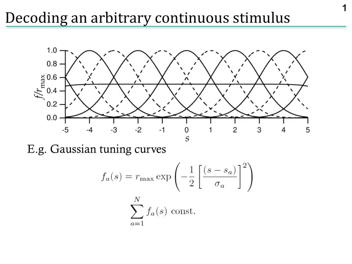
E.g. Gaussian tuning curves

Decoding an arbitrary continuous stimulus

.. what is P(ra|s)?

1

Many neurons “voting” for an outcome. Work through a specific example

• assume independence
• assume Poisson firing

Noise model: Poisson distribution PT[k] = (lT)k exp(-lT)/k!

Decoding an arbitrary continuous stimulus

2

Assume Poisson: Assume independent:

Population response of 11 cells with Gaussian tuning curves

Need to know full P[r|s]

3

Apply ML: maximize ln P[r|s] with respect to s Set derivative to zero, use sum = constant From Gaussianity of tuning curves, If all s same

ML

4

Apply MAP: maximise ln p[s|r] with respect to s Set derivative to zero, use sum = constant From Gaussianity of tuning curves,

MAP

5

Given this data:

Constant prior Prior with mean -2, variance 1

MAP:

6

For stimulus s, have estimated sest Bias: Cramer-Rao bound: Mean square error: Variance:

Fisher information

(ML is unbiased: b = b’ = 0)

How good is our estimate?

7

Alternatively: Quantifies local stimulus discriminability

Fisher information

8

Entropy and Shannon information

9

For a random variable X with distribution p(x), the entropy is H[X] = - Sx p(x) log2p(x) Information is defined as I[X] = - log2p(x)

Entropy and Shannon information

10

Mutual Information between X and Y is defined as

MI[X,Y] = H[X] - E [H[X|Y=y]] = H[Y] - E [H[Y|X=x]]

y x

How much information does a single spike convey about the stimulus? Key idea: the information that a spike gives about the stimulus is the reduction in entropy between the distribution of spike times not knowing the stimulus, and the distribution of times knowing the stimulus. The response to an (arbitrary) stimulus sequence s is r(t). Without knowing that the stimulus was s, the probability of observing a spike in a given bin is proportional to , the mean rate, and the size of the bin. Consider a bin Dt small enough that it can only contain a single spike. Then in the bin at time t,

Information in single spikes

11

Now compute the entropy difference: , Assuming , and using In terms of information per spike (divide by ): Note substitution of a time average for an average over the r ensemble. ß prior ß conditional

Information in single spikes

12

• p

We can use the information about the stimulus to evaluate our reduced dimensionality models.

Using information to evaluate neural models

13

Mutual information is a measure of the reduction of uncertainty about one quantity that is achieved by observing another. Uncertainty is quantified by the entropy of a probability distribution, ∑ p(x) log2 p(x). We can compute the information in the spike train directly, without direct reference to the stimulus (Brenner et al., Neural Comp., 2000) This sets an upper bound on the performance of the model. Repeat a stimulus of length T many times and compute the time-varying rate r(t), which is the probability of spiking given the stimulus.

Evaluating models using information

14

Information in timing of 1 spike: By definition

Evaluating models using information

15

Given: By definition Bayes’ rule

Evaluating models using information

16

Given: By definition Bayes’ rule Dimensionality reduction

Evaluating models using information

17

Given: By definition So the information in the K-dimensional model is evaluated using the distribution of projections: Bayes’ rule Dimensionality reduction

Evaluating models using information

18

Here we used information to evaluate reduced models of the Hodgkin-Huxley neuron. 1D: STA only 2D: two covariance modes Twist model

Using information to evaluate neural models

19

6 4 2

Information in E-Vector (bits)

6 4 2

Information in STA (bits) Mode 1 Mode 2

The STA is the single most informative dimension.

Information in 1D

20

• The information is related to the eigenvalue of the corresponding eigenmode
• Negative eigenmodes are much more informative
• Information in STA and leading negative eigenmodes up to 90% of the total

1.0 0.8 0.6 0.4 0.2 0.0

Information fraction

3 2 1

• 1

Eigenvalue (normalised to stimulus variance)

Information in 1D

21

• We recover significantly more information from a 2-dimensional description

1.0 0.8 0.6 0.4 0.2 0.0

Information about two features (normalized)

1.0 0.8 0.6 0.4 0.2 0.0

Information about STA (normalized)

Information in 2D

22

How can one compute the entropy and information of spike trains? Entropy:

Strong et al., 1997; Panzeri et al. Discretize the spike train into binary words w with letter size Dt, length T. This takes into account correlations between spikes on timescales TDt. Compute pi = p(wi), then the naïve entropy is

Calculating information in spike trains

23

Information : difference between the variability driven by stimuli and that due to noise. Take a stimulus sequence s and repeat many times. For each time in the repeated stimulus, get a set of words P(w|s(t)). Average over s à average over time: Hnoise = < H[P(w|si)] >i. Choose length of repeated sequence long enough to sample the noise entropy adequately. Finally, do as a function of word length T and extrapolate to infinite T.

Reinagel and Reid, ‘00

Calculating information in spike trains

24

Fly H1:

• btain information rate of

~80 bits/sec or 1-2 bits/spike.

Calculating information in spike trains

25

Another example: temporal coding in the LGN (Reinagel and Reid ‘00)

Calculating information in the LGN

26

Apply the same procedure: collect word distributions for a random, then repeated stimulus.

Calculating information in the LGN

27

Use this to quantify how precise the code is, and over what timescales correlations are important.

Information in the LGN

28