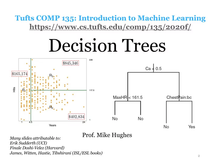
Decision Trees Prof. Mike Hughes Many slides attributable to: Erik - PowerPoint PPT Presentation

Tufts COMP 135: Introduction to Machine Learning https://www.cs.tufts.edu/comp/135/2020f/ Decision Trees Prof. Mike Hughes Many slides attributable to: Erik Sudderth (UCI) Finale Doshi-Velez (Harvard) James, Witten, Hastie, Tibshirani (ISL/ESL books) 2

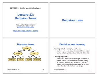
Objectives for day 14 Decision Trees • Decision Tree Regression • How to predict • How to train • Greedy recursive algorithm • Possible cost functions • Decision Tree Classification • Possible cost functions • Comparisons to other methods Mike Hughes - Tufts COMP 135 - Spring 2019 3

What will we learn? Evaluation Supervised Training Learning Data, Label Pairs Performance { x n , y n } N measure Task n =1 Unsupervised Learning data label x y Reinforcement Learning Prediction Mike Hughes - Tufts COMP 135 - Spring 2019 4

Task: Regression y is a numeric variable Supervised e.g. sales in $$ Learning regression y Unsupervised Learning Reinforcement Learning x Mike Hughes - Tufts COMP 135 - Spring 2019 5

Salary prediction for Hitters data Mike Hughes - Tufts COMP 135 - Spring 2019 6

Salary Prediction by “Region” Divide x space into regions, predict constant within each region Regions are rectangular (“axis aligned”) Mike Hughes - Tufts COMP 135 - Spring 2019 7

From Regions to Decision Tree Mike Hughes - Tufts COMP 135 - Spring 2019 8

Decision tree regression Classification and Regression Trees by Breiman et al (1984) Parameters: - tree architecture (list of nodes, list of parent-child pairs) - at each internal node: x variable id and threshold value - at each leaf: scalar y value to predict Hyperparameters - max_depth, min_samples_split Prediction procedure: - Determine which leaf (region) the input features belong to - Guess the y value associated with that leaf Training procedure: - minimize error on training set - use greedy heuristics (build from root to leaf) Mike Hughes - Tufts COMP 135 - Spring 2019 9

Ideal Training for Decision Tree J X X y R j ) 2 min ( y n − ˆ R 1 ,...R J j =1 n : x n ∈ R j Search space is too big (so many regions)! Hard to solve exactly… … let’s break it down into subproblems Mike Hughes - Tufts COMP 135 - Spring 2019 10

Key subproblem: Within 1 region, how to find best binary split? Given a big region R, find the best possible binary split into two subregions (best means minimize mean squared error) min j,s, ˆ y R 1 , ˆ y R 2 We can solve this subproblem efficiently! For each feature index j in 1, 2, … F: - find its best possible cut point s[j] and its cost[j] j <- argmin( cost[1] … cost[F] ) return best index j and its cut point s[j] Let binary_split denote this procedure Mike Hughes - Tufts COMP 135 - Spring 2019 11

Greedy top-down training Hyperparameters controling complexity Training is a recursive process. - MAX_DEPTH Returns a tree (by reference to its root node) - MIN_INTERNAL_NODE_SIZE - MIN_LEAF_NODE_SIZE def train_tree_greedy (x_NF, y_N, depth d): if d >= MAX_DEPTH : return LeafNode(x_NF, y_N) elif N < MIN_INTERNAL_NODE_SIZE : return LeafNode(x_NF, y_N) else: # j : integer index indicating feature to split # s : real value used as threshold to split # L / R : number of examples in left / right region j, s, x_LF, x_RF, y_L, y_R = binary_split (x_NF, y_N) if no split possible : return LeafNode(x_NF, y_N) left_child = train_tree_greedy (x_LF, y_L, d+1) right_child = train_tree_greedy (x_RF, y_R, d+1) return InternalNode( x_NF, y_N , j, s, left_child, right_child) Mike Hughes - Tufts COMP 135 - Spring 2019 12

Greedy Tree for Hitters Data Mike Hughes - Tufts COMP 135 - Spring 2019 13

<latexit sha1_base64="dJ1fREy7huDN7QkHSqYPu5HWjo=">ACG3icbVBNS8NAEN34bf2qevSyWAS9lKQKiCIXjyq2Co0JWy203bpZhN2J2I+R9e/CtePCjiSfDgv3Fbe9Dqgxke782wOy9MpDoup/OxOTU9Mzs3HxpYXFpeaW8utYwcao51HksY30TMgNSKijQAk3iQYWhRKuw/7pwL+BW1ErK4wS6AVsa4SHcEZWiko1/wewzwrgvyoEfUR7jDPIK2YKrYpn6eBYIe0jvbfaHopV/QnaBcavuEPQv8UakQkY4D8rvfjvmaQKuWTGND03wVbONAouoSj5qYGE8T7rQtNSxSIwrXx4W0G3rNKmnVjbUkiH6s+NnEXGZFoJyOGPTPuDcT/vGaKnYNWLlSIij+/VAnlRjOgiKtoUGjKzhHEt7F8p7zHNONo4SzYEb/zkv6Rq3q71drFXuX4ZBTHNkgm2SbeGSfHJMzck7qhJN78kieyYvz4Dw5r87b9+iEM9pZJ7/gfHwBcaegWw=</latexit> <latexit sha1_base64="yH1TQDUBZkWkXyE1I4qvKwaSocs=">ACHXicbVDLSgMxFM34rPVdekmWARXZaYWFEounFZi31ApwyZNOGZjJDkhGHdH7Ejb/ixoUiLtyIf2P6WGjrgcDhnHO5ucePGZXKtr+tpeWV1bX13EZ+c2t7Z7ewt9+USIwaeCIRaLtI0kY5aShqGKkHQuCQp+Rlj+8HvuteyIkjfidSmPSDVGf04BipIzkFSruACmdZp6uZ/ASuoFAWDuZHtVHGXRlEnqawgv4FHoUg5NKPWoVyjaJXsCuEicGSmCGWpe4dPtRTgJCVeYISk7jh2rkZCUcxIlncTSWKEh6hPOoZyFBLZ1ZPrMnhslB4MImEeV3Ci/p7QKJQyDX2TDJEayHlvLP7ndRIVnHc15XGiCMfTRUHCoIrguCrYo4JgxVJDEBbU/BXiATIFKVNo3pTgzJ+8SJrlknNaKt9WitWrWR05cAiOwAlwBmoghtQAw2AwSN4Bq/gzXqyXqx362MaXbJmMwfgD6yvH9r0obs=</latexit> Cost functions for regression trees • Mean squared error • Assumed on previous slides, very common • How to solve for region’s best guess? Optimal solution: min Guess mean output value of the region: min 1 s, ˆ y R 1 , X y R = y i ˆ | R | i : x i ∈ R • Mean absolute error • Possible! (supported in sklearn) • How to solve for region’s best guess? Optimal solution: Guess median output value of the region: y R = median( { y i : x i ∈ R } ) ˆ Mike Hughes - Tufts COMP 135 - Spring 2019 14

Task: Binary Classification y is a binary variable Supervised (red or blue) Learning binary classification x 2 Unsupervised Learning Reinforcement Learning x 1 Mike Hughes - Tufts COMP 135 - Spring 2019 15

Decision Tree Classifier Goal: Does patient have heart disease? Leaves make binary predictions! Mike Hughes - Tufts COMP 135 - Spring 2019 16

Decision Tree Probabilistic Classifier Goal: What probability does patient have heart disease? + + - - +++ + - - 0.667 0.5 + + ++ - + - - - 0.25 0.80 Leaves count samples in each class! Then return fractions! Mike Hughes - Tufts COMP 135 - Spring 2019 17

Decision Tree Classifier Classification and Regression Trees by Breiman et al (1984) Parameters: - tree architecture (list of nodes, list of parent-child pairs) - at each internal node: x variable id and threshold - at each leaf: number of examples in each class Hyperparameters: - max_depth, min_samples_split Prediction: - identify rectangular region for input x - predict : most common label value in region - predict_proba : fraction of each label in region Training: - minimize cost on training set - greedy construction from root to leaf 18

<latexit sha1_base64="JAZ0vg9+DgsaS9yITSICD1psF2c=">ACJ3icbZDLSgMxFIYzXmu9V26CRahBS0zVCESrEbV1LBXqCtQyZN29DMheSMtAzNm58FTeCiujSNzG9LT1h8DHf87h5PxOILgC0/wyFhaXldWE2vJ9Y3Nre3Uzm5V+aGkrEJ94cu6QxQT3GMV4CBYPZCMuI5gNadfGtVrD0wq7nt3MAxYyVdj3c4JaAtO3XZBDaAiPoK4gwe2JF1cRMf4eEcBYXcFOFrh3RghXfl3CgKcYZCx9rpFk7lTZz5lh4HqwpNFUZTv12mz7NHSZB1QpRqWGUArIhI4FSxONkPFAkL7pMsaGj3iMtWKxnfG+FA7bdzxpX4e4LH7eyIirlJD19GdLoGemq2NzP9qjRA6562Ie0EIzKOTRZ1QYPDxKDTc5pJREMNhEqu/4pj0hCQUeb1CFYsyfPQzWfs05y+dvTdPFqGkcC7aMDlEWOkNFdI3KqIoekTP6A29G0/Gi/FhfE5aF4zpzB76I+P7B9BFo10=</latexit> <latexit sha1_base64="rZTIAaWf/chI2mkSUD6vFXOvwR0=">ACZnicbZHPa9RAFMcn8Ve7al1bxIOXh4uwhbokVCEQrEXT1LBbQubNUwmL9uhk5nszIs0hPyT3jx78c9wdrMHbX0w8Jnv+zEz38kqJR1F0c8gvHP3v0HW9uDh48e7zwZPt09c6a2AqfCKGMvMu5QSY1TkqTworLIy0zheXZ1sqf0frpNFfqalwXvKFloUnLyUDruE8JpaYRx1Y7hO2/jD5+4Amh5gH47gNSuLtNWHMXdtxOoPHWQKLPo8QCS5bLmud8JSMhKrhcKl5AUlos27lo/ph+gPeSoiK/axk2q9PhKJpE64DbEG9gxDZxmg5/JLkRdYmahOLOzeKonLUmhsBsktcOKiyu+wJlHzUt083ZtUwevJDYaxfmCt/t3R8tK5psx8Zcnp0t3MrcT/5WY1Fe/nrdRVTahFf1BRKyADK8hlxYFqcYDF1b6u4K45N4e8j8z8CbEN598G84OJ/GbyeGXt6Pjxs7tgL9pKNWczesWP2iZ2yKRPsV7Ad7AZ7we9wJ3wWPu9Lw2DTs8f+iRD+ACEKtzs=</latexit> Cost functions for classification trees • Information gain or “entropy” • Cost for a region with N examples of C classes C p c , 1 X X cost( x 1: N , y 1: N ) = − p c log p c , δ c ( y n ) N n c =1 • Gini impurity C X cost( x 1: N , y 1: N ) = p c (1 − p c ) c =1 Mike Hughes - Tufts COMP 135 - Spring 2019 19

Advantages of Decision Trees + Can handle heterogeneous datasets (some features are numerical, some are categorical) easily without requiring standardized scales like penalized linear models do + Flexible non-linear decision boundaries + Relatively few hyperparameters to select Mike Hughes - Tufts COMP 135 - Spring 2019 20

Limitations of Decision Trees Axis-aligned assumption not always a good idea Mike Hughes - Tufts COMP 135 - Spring 2019 21

Summary of Classifiers Knobs to tune Function Interpret? class flexibility Logistic L2/L1 penalty on Linear Inspect Regression weights weights MLPClassifier Universal Challenging L2/L1 penalty on weights Num layers, num units (with Activation functions enough GD method: SGD or LBFGS or … units) Step size, batch size K Nearest Number of Neighbors Piecewise Inspect Neighbors Distance metric constant neighbors Classifier Decision Max. depth Axis-aligned Inspect Tree Min. leaf size Piecewise tree Classifier constant Mike Hughes - Tufts COMP 135 - Spring 2019 22