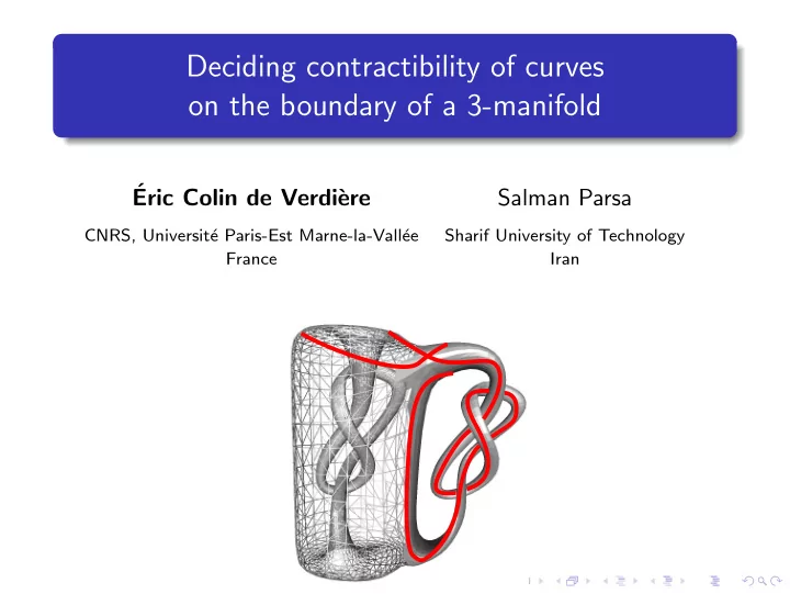
SLIDE 1 Deciding contractibility of curves
- n the boundary of a 3-manifold
´ Eric Colin de Verdi` ere
CNRS, Universit´ e Paris-Est Marne-la-Vall´ ee France
Salman Parsa
Sharif University of Technology Iran
SLIDE 2
The problem
Given solid obstacles in R3, and a closed curve c on the boundary of one obstacle, decide whether c can be shrunk continuously into a point in the complement M of the obstacles. ( = is contractible in M = is homotopic to a point in M) More generally, M is a triangulated 3-manifold with boundary.
SLIDE 3
The problem
Given solid obstacles in R3, and a closed curve c on the boundary of one obstacle, decide whether c can be shrunk continuously into a point in the complement M of the obstacles. ( = is contractible in M = is homotopic to a point in M) More generally, M is a triangulated 3-manifold with boundary.
SLIDE 4
The problem
Given solid obstacles in R3, and a closed curve c on the boundary of one obstacle, decide whether c can be shrunk continuously into a point in the complement M of the obstacles. ( = is contractible in M = is homotopic to a point in M) More generally, M is a triangulated 3-manifold with boundary.
SLIDE 5
The problem
Given solid obstacles in R3, and a closed curve c on the boundary of one obstacle, decide whether c can be shrunk continuously into a point in the complement M of the obstacles. ( = is contractible in M = is homotopic to a point in M) More generally, M is a triangulated 3-manifold with boundary.
SLIDE 6
The problem
Given solid obstacles in R3, and a closed curve c on the boundary of one obstacle, decide whether c can be shrunk continuously into a point in the complement M of the obstacles. ( = is contractible in M = is homotopic to a point in M) More generally, M is a triangulated 3-manifold with boundary.
SLIDE 7
The problem
Given solid obstacles in R3, and a closed curve c on the boundary of one obstacle, decide whether c can be shrunk continuously into a point in the complement M of the obstacles. ( = is contractible in M = is homotopic to a point in M) More generally, M is a triangulated 3-manifold with boundary.
SLIDE 8 The problem
Image by Tamal Dey and students
Given solid obstacles in R3, and a closed curve c on the boundary of one obstacle, decide whether c can be shrunk continuously into a point in the complement M of the obstacles. ( = is contractible in M = is homotopic to a point in M) More generally, M is a triangulated 3-manifold with boundary.
SLIDE 9 The problem
Image by Tamal Dey and students
Given solid obstacles in R3, and a closed curve c on the boundary of one obstacle, decide whether c can be shrunk continuously into a point in the complement M of the obstacles. ( = is contractible in M = is homotopic to a point in M) More generally, M is a triangulated 3-manifold with boundary.
SLIDE 10 The problem
Image by Tamal Dey and students
Given solid obstacles in R3, and a closed curve c on the boundary of one obstacle, decide whether c can be shrunk continuously into a point in the complement M of the obstacles. ( = is contractible in M = is homotopic to a point in M) More generally, M is a triangulated 3-manifold with boundary.
SLIDE 11 Testing contractibility in manifolds: known results
Manifolds M is an arbitrary compact, triangulated d-manifold with boundary (each point of M has a neighborhood homeomorphic to the d-dimensional open ball or unit half-ball). Known results for testing contractibility of curves in M 2-manifolds (=surfaces): solvable in linear time [Dey and Guha,
1999]; [Lazarus and Rivaud, 2012]; [Erickson and Whittlesey, 2013];
3-manifolds: decidable via automatic group theory [Epstein,
1992]. . . but no explicit complexity bound, and best known
algorithm is at least triply exponential; 4-manifolds: undecidable [Novikov, 1955].
SLIDE 12 Testing contractibility in manifolds: known results
Manifolds M is an arbitrary compact, triangulated d-manifold with boundary (each point of M has a neighborhood homeomorphic to the d-dimensional open ball or unit half-ball). Known results for testing contractibility of curves in M 2-manifolds (=surfaces): solvable in linear time [Dey and Guha,
1999]; [Lazarus and Rivaud, 2012]; [Erickson and Whittlesey, 2013];
3-manifolds: decidable via automatic group theory [Epstein,
1992]. . . but no explicit complexity bound, and best known
algorithm is at least triply exponential; 4-manifolds: undecidable [Novikov, 1955].
SLIDE 13 Testing contractibility in manifolds: known results
Manifolds M is an arbitrary compact, triangulated d-manifold with boundary (each point of M has a neighborhood homeomorphic to the d-dimensional open ball or unit half-ball). Known results for testing contractibility of curves in M 2-manifolds (=surfaces): solvable in linear time [Dey and Guha,
1999]; [Lazarus and Rivaud, 2012]; [Erickson and Whittlesey, 2013];
3-manifolds: decidable via automatic group theory [Epstein,
1992]. . . but no explicit complexity bound, and best known
algorithm is at least triply exponential; 4-manifolds: undecidable [Novikov, 1955].
SLIDE 14 Testing contractibility in manifolds: known results
Manifolds M is an arbitrary compact, triangulated d-manifold with boundary (each point of M has a neighborhood homeomorphic to the d-dimensional open ball or unit half-ball). Known results for testing contractibility of curves in M 2-manifolds (=surfaces): solvable in linear time [Dey and Guha,
1999]; [Lazarus and Rivaud, 2012]; [Erickson and Whittlesey, 2013];
3-manifolds: decidable via automatic group theory [Epstein,
1992]. . . but no explicit complexity bound, and best known
algorithm is at least triply exponential; 4-manifolds: undecidable [Novikov, 1955].
SLIDE 15
Our result
Theorem There is an algorithm that takes as input: a triangulated 3-manifold with boundary M, with t tetrahedra, a polygonal curve c on @M with n edges and m self-crossings, and decides whether c is contractible in M in time 2O((t+n+m)2). c may be non-simple (=may have self-crossings). We assume that c is in general position on @M.
SLIDE 16 Roadmap of the talk
1 The case where c is simple:
Strong relation to the Unknot problem. (Digression:) An algorithm for this case.
2 An algorithm under a simplifying assumption. 3 The algorithm.
SLIDE 17
The Unknot problem, and the case of simple curves
SLIDE 18 The Unknot problem
The Unknot problem Given a polygonal closed curve K in R3 that is simple, determine whether K is unknotted. Theorem [Hass, Lagarias, Pippenger, 1999] The Unknot problem is in NP (thus solvable in exponential time).
Remark: also in co-NP [Lackenby, 2016], but not known to be in P!
Sketch of proof Let M be obtained from R3 by removing a neighborhood of K, and let c be a certain simple curve on @M “parallel” to K. K unknotted ⇔ K bounds a disk in R3 ⇔ c bounds a disk in M. Goal: Polynomial-size certificate that c bounds a disk in M.
SLIDE 19 The Unknot problem
The Unknot problem Given a polygonal closed curve K in R3 that is simple, determine whether K is unknotted. Theorem [Hass, Lagarias, Pippenger, 1999] The Unknot problem is in NP (thus solvable in exponential time).
Remark: also in co-NP [Lackenby, 2016], but not known to be in P!
Sketch of proof Let M be obtained from R3 by removing a neighborhood of K, and let c be a certain simple curve on @M “parallel” to K. K unknotted ⇔ K bounds a disk in R3 ⇔ c bounds a disk in M. Goal: Polynomial-size certificate that c bounds a disk in M.
SLIDE 20 The Unknot problem
The Unknot problem Given a polygonal closed curve K in R3 that is simple, determine whether K is unknotted. Theorem [Hass, Lagarias, Pippenger, 1999] The Unknot problem is in NP (thus solvable in exponential time).
Remark: also in co-NP [Lackenby, 2016], but not known to be in P!
Sketch of proof Let M be obtained from R3 by removing a neighborhood of K, and let c be a certain simple curve on @M “parallel” to K. K unknotted ⇔ K bounds a disk in R3 ⇔ c bounds a disk in M. Goal: Polynomial-size certificate that c bounds a disk in M.
SLIDE 21 The Unknot problem
The Unknot problem Given a polygonal closed curve K in R3 that is simple, determine whether K is unknotted. Theorem [Hass, Lagarias, Pippenger, 1999] The Unknot problem is in NP (thus solvable in exponential time).
Remark: also in co-NP [Lackenby, 2016], but not known to be in P!
Sketch of proof Let M be obtained from R3 by removing a neighborhood of K, and let c be a certain simple curve on @M “parallel” to K. K unknotted ⇔ K bounds a disk in R3 ⇔ c bounds a disk in M. Goal: Polynomial-size certificate that c bounds a disk in M.
SLIDE 22 The Unknot problem
The Unknot problem Given a polygonal closed curve K in R3 that is simple, determine whether K is unknotted. Theorem [Hass, Lagarias, Pippenger, 1999] The Unknot problem is in NP (thus solvable in exponential time).
Remark: also in co-NP [Lackenby, 2016], but not known to be in P!
Sketch of proof Let M be obtained from R3 by removing a neighborhood of K, and let c be a certain simple curve on @M “parallel” to K. K unknotted ⇔ K bounds a disk in R3 ⇔ c bounds a disk in M. Goal: Polynomial-size certificate that c bounds a disk in M.
SLIDE 23 The Unknot problem
The Unknot problem Given a polygonal closed curve K in R3 that is simple, determine whether K is unknotted. Theorem [Hass, Lagarias, Pippenger, 1999] The Unknot problem is in NP (thus solvable in exponential time).
Remark: also in co-NP [Lackenby, 2016], but not known to be in P!
Sketch of proof Let M be obtained from R3 by removing a neighborhood of K, and let c be a certain simple curve on @M “parallel” to K. K unknotted ⇔ K bounds a disk in R3 ⇔ c bounds a disk in M. Goal: Polynomial-size certificate that c bounds a disk in M.
SLIDE 24 The Unknot problem
The Unknot problem Given a polygonal closed curve K in R3 that is simple, determine whether K is unknotted. Theorem [Hass, Lagarias, Pippenger, 1999] The Unknot problem is in NP (thus solvable in exponential time).
Remark: also in co-NP [Lackenby, 2016], but not known to be in P!
Sketch of proof Let M be obtained from R3 by removing a neighborhood of K, and let c be a certain simple curve on @M “parallel” to K. K unknotted ⇔ K bounds a disk in R3 ⇔ c bounds a disk in M. Goal: Polynomial-size certificate that c bounds a disk in M.
SLIDE 25
Side remark: The na¨ ıve encoding does not work [Snoeyink, 1990]
A knot with no polynomial-size spanning disk.
SLIDE 26
Side remark: Normal surfaces in M [Haken, 1961]
1 2 4 3 5 6 7 A surface embedded in M is normal if its intersection with each tetrahedron of M is the disjoint union of triangles and quads. There are 4 types of triangles and 3 types of quads per tetrahedron.
SLIDE 27 Side remark: Normal surfaces in M [Haken, 1961]
1 2 4 3 5 6 7 A surface embedded in M is normal if its intersection with each tetrahedron of M is the disjoint union of triangles and quads. There are 4 types of triangles and 3 types of quads per tetrahedron. Normal coordinates A normal surface S can be encoded by a vector [S ] ∈ Z7t such that:
the numbers of arcs of each type at the interface between two tetrahedra match (matching equations); for each tetrahedron, at least two of the quad coordinates are zero (quadrilateral constraints).
Conversely, each such vector in Z7t corresponds to a normal surface.
SLIDE 28 Side remark: The certificate (very high-level view)
1 If c bounds a disk, it bounds a normal disk 2 . . . actually, a fundamental normal disk S , such that
([S ] = [S 0] + [S 00]) = ⇒ (S 0 = ∅ or S 00 = ∅).
3 Every fundamental normal disk has coordinates ≤ 2O(t). 4 Given normal coordinates, one can check whether they
correspond to a normal disk bounding c in polynomial time. Some ingredients
1 surgery, 2 is linear in the normal coordinates, 3 algebra, polyhedral cone of vectors in Z7t satisfying the
matching equations,
4 ad hoc connectivity test.
SLIDE 29 Side remark: The certificate (very high-level view)
1 If c bounds a disk, it bounds a normal disk 2 . . . actually, a fundamental normal disk S , such that
([S ] = [S 0] + [S 00]) = ⇒ (S 0 = ∅ or S 00 = ∅).
3 Every fundamental normal disk has coordinates ≤ 2O(t). 4 Given normal coordinates, one can check whether they
correspond to a normal disk bounding c in polynomial time. Some ingredients
1 surgery, 2 is linear in the normal coordinates, 3 algebra, polyhedral cone of vectors in Z7t satisfying the
matching equations,
4 ad hoc connectivity test.
SLIDE 30
Contractibility algorithm, if c is simple
Dehn’s lemma Let c be a simple closed curve in @M. Then c is contractible in M iff it bounds a disk in M. Key consequences of the previous slide c bounds a disk if and only if it bounds a normal disk with coordinates ≤ 2O(t). Given normal coordinates, one can check whether they correspond to a normal disk bounded by c in polynomial time. Morals Our contractibility problem is solved (in exponential time) in the case where c is simple. Any subexponential algorithm for our problem would imply a subexponential algorithm for Unknot.
SLIDE 31
Non-simple curves
SLIDE 32 Overall strategy
Very basic idea Split c into simple closed curves. Main inspiration Reuse the techniques of the proof of Dehn’s lemma, or its extension, the loop theorem [Papakyriakopoulos, 1957]:
If there is a curve on @M then there is a curve on @M not contractible on @M not contractible on @M but contractible on M, but bounding a disk in M (and thus simple).
SLIDE 33
If c is contractible. . .
. . . it bounds a (possibly) self-intersecting disk, which we can choose in general position. One can get several types of singularities: double curve triple point branchpoint
SLIDE 34
If c is contractible. . .
. . . it bounds a (possibly) self-intersecting disk, which we can choose in general position. One can get several types of singularities: double curve triple point branchpoint handled later handled later
SLIDE 35
If c is contractible. . .
. . . it bounds a (possibly) self-intersecting disk, which we can choose in general position. One can get several types of singularities: double curve triple point branchpoint handled later handled later c is strongly contractible if it bounds a disk with only double curves as singularities.
SLIDE 36
Types of double curves
double closed curve (easy to get rid of) double arc
SLIDE 37
Types of double curves
double closed curve (easy to get rid of) double arc
SLIDE 38
Types of double curves
double closed curve (easy to get rid of) double arc c can be contractible and not strongly contractible (e.g., with an odd number of self-crossings).
SLIDE 39
Toy problem: only double curves
SLIDE 40 Removing a double arc
c
α β γ δ
c0
α γ
c00
α β γ δ
Choose two self-crossings of c, splitting c into ↵ · · · . Let c0 = ↵ · and c00 = ↵ · 1 · · 1. c is homotopic to c0 · 1 · (c001 · c0) · . Two crucial properties
1 For all choices of the self-crossings, if c0 and c00 are
contractible closed curves, then c is contractible.
2 If c is strongly contractible, then for some choice of the
self-crossings, each of c0 and c00 is strongly contractible.
SLIDE 41 Removing a double arc
c
α β γ δ
c0
α γ
c00
α β γ δ
Choose two self-crossings of c, splitting c into ↵ · · · . Let c0 = ↵ · and c00 = ↵ · 1 · · 1. c is homotopic to c0 · 1 · (c001 · c0) · . Two crucial properties
1 For all choices of the self-crossings, if c0 and c00 are
contractible closed curves, then c is contractible.
2 If c is strongly contractible, then for some choice of the
self-crossings, each of c0 and c00 is strongly contractible.
SLIDE 42 Removing a double arc
c
α β γ δ
c0
α γ
c00
α β γ δ
Choose two self-crossings of c, splitting c into ↵ · · · . Let c0 = ↵ · and c00 = ↵ · 1 · · 1. c is homotopic to c0 · 1 · (c001 · c0) · . Two crucial properties
1 For all choices of the self-crossings, if c0 and c00 are
contractible closed curves, then c is contractible.
2 If c is strongly contractible, then for some choice of the
self-crossings, each of c0 and c00 is strongly contractible.
SLIDE 43 Removing a double arc
c
α β γ δ
c0
α γ
c00
α β γ δ
Choose two self-crossings of c, splitting c into ↵ · · · . Let c0 = ↵ · and c00 = ↵ · 1 · · 1. c is homotopic to c0 · 1 · (c001 · c0) · . Two crucial properties
1 For all choices of the self-crossings, if c0 and c00 are
contractible closed curves, then c is contractible.
2 If c is strongly contractible, then for some choice of the
self-crossings, each of c0 and c00 is strongly contractible.
SLIDE 44 Removing a double arc
c
α β γ δ
c0
α γ
c00
α β γ δ
Choose two self-crossings of c, splitting c into ↵ · · · . Let c0 = ↵ · and c00 = ↵ · 1 · · 1. c is homotopic to c0 · 1 · (c001 · c0) · . Two crucial properties
1 For all choices of the self-crossings, if c0 and c00 are
contractible closed curves, then c is contractible.
2 If c is strongly contractible, then for some choice of the
self-crossings, each of c0 and c00 is strongly contractible.
SLIDE 45 An algorithm
Two crucial properties
1
For all choices of the self-crossings, if c0 and c00 are contractible closed curves, then c is contractible.
2
If c is strongly contractible, then for some choice of the self-crossings, each of c0 and c00 is strongly contractible.
Input: closed curve c Output: ⇢ (1) “c is contractible” OR (2) “c is not strongly contractible”. Algorithm Sub(c) If c has an odd number of self-crossings, return 2. If c has no self-crossing: Determine if c is contractible (see previous slides). If yes, return 1. If no, return 2. For each choice of two self-crossing points of c:
compute the associated curves c0 and c00; if Sub(c0)=1 and Sub(c00)=1 then return 1.
Return 2.
SLIDE 46 An algorithm
Two crucial properties
1
For all choices of the self-crossings, if c0 and c00 are contractible closed curves, then c is contractible.
2
If c is strongly contractible, then for some choice of the self-crossings, each of c0 and c00 is strongly contractible.
Input: closed curve c Output: ⇢ (1) “c is contractible” OR (2) “c is not strongly contractible”. Algorithm Sub(c) If c has an odd number of self-crossings, return 2. If c has no self-crossing: Determine if c is contractible (see previous slides). If yes, return 1. If no, return 2. For each choice of two self-crossing points of c:
compute the associated curves c0 and c00; if Sub(c0)=1 and Sub(c00)=1 then return 1.
Return 2.
SLIDE 47 An algorithm
Two crucial properties
1
For all choices of the self-crossings, if c0 and c00 are contractible closed curves, then c is contractible.
2
If c is strongly contractible, then for some choice of the self-crossings, each of c0 and c00 is strongly contractible.
Input: closed curve c Output: ⇢ (1) “c is contractible” OR (2) “c is not strongly contractible”. Algorithm Sub(c) If c has an odd number of self-crossings, return 2. If c has no self-crossing: Determine if c is contractible (see previous slides). If yes, return 1. If no, return 2. For each choice of two self-crossing points of c:
compute the associated curves c0 and c00; if Sub(c0)=1 and Sub(c00)=1 then return 1.
Return 2.
SLIDE 48
General case
SLIDE 49
Two-sheeted covering spaces
Definition Continuous map ⇡ : ˜ X → X such that: ⇡ is a local homeomorphism (can “lift” paths or homotopies from X to ˜ X), ⇡ is two-to-one. Why can it be useful? Intuition: when projecting, only double points can be created (no triple points, no branchpoint).
SLIDE 50
Two-sheeted covering spaces
Definition Continuous map ⇡ : ˜ X → X such that: ⇡ is a local homeomorphism (can “lift” paths or homotopies from X to ˜ X), ⇡ is two-to-one. Why can it be useful? Intuition: when projecting, only double points can be created (no triple points, no branchpoint).
SLIDE 51
Two-sheeted covering spaces
Definition Continuous map ⇡ : ˜ X → X such that: ⇡ is a local homeomorphism (can “lift” paths or homotopies from X to ˜ X), ⇡ is two-to-one. Why can it be useful? Intuition: when projecting, only double points can be created (no triple points, no branchpoint).
SLIDE 52
Two-sheeted covering spaces
Definition Continuous map ⇡ : ˜ X → X such that: ⇡ is a local homeomorphism (can “lift” paths or homotopies from X to ˜ X), ⇡ is two-to-one. Why can it be useful? Intuition: when projecting, only double points can be created (no triple points, no branchpoint).
SLIDE 53 Key construction of the loop theorem
Proposition Assume c is contractible. Let f : D → M be a self-intersecting disk such that f |@D = c. c D @M Then f can be expressed as a composition in a tower of covering spaces:
D → Vp , → Mp → Vp1 , → Mp1 . . . V1 , → M1 → V0 , → M0 = M, and
each map Mi+1 → Vi is a two-sheeted cover, each map D → Vi sends @D to @Vi, @Vp is a disjoint union of spheres. c is virtually strongly contractible if there is a tower such that D → Vp has only double curves as singularities.
SLIDE 54 Key construction of the loop theorem
Proposition Assume c is contractible. Let f : D → M be a self-intersecting disk such that f |@D = c. c D @M Then f can be expressed as a composition in a tower of covering spaces:
D → Vp , → Mp → Vp1 , → Mp1 . . . V1 , → M1 → V0 , → M0 = M, and
each map Mi+1 → Vi is a two-sheeted cover, each map D → Vi sends @D to @Vi, @Vp is a disjoint union of spheres. c is virtually strongly contractible if there is a tower such that D → Vp has only double curves as singularities.
SLIDE 55 Key construction of the loop theorem
Proposition Assume c is contractible. Let f : D → M be a self-intersecting disk such that f |@D = c. c D @M Then f can be expressed as a composition in a tower of covering spaces:
D → Vp , → Mp → Vp1 , → Mp1 . . . V1 , → M1 → V0 , → M0 = M, and
each map Mi+1 → Vi is a two-sheeted cover, each map D → Vi sends @D to @Vi, @Vp is a disjoint union of spheres. c is virtually strongly contractible if there is a tower such that D → Vp has only double curves as singularities.
SLIDE 56 Virtually strongly contractible curves
If c is contractible, the self-intersecting disk D ! M expresses as D ! Vp , ! Mp ! Vp1 , ! Mp1 . . . V1 , ! M1 ! V0 , ! M0 = M.
SLIDE 57 Virtually strongly contractible curves
If c is contractible, the self-intersecting disk D ! M expresses as D ! Vp , ! Mp ! Vp1 , ! Mp1 . . . V1 , ! M1 ! V0 , ! M0 = M.
Two crucial properties for a non-simple curve c
1 For all choices of the self-crossings, if c0 and c00 are
contractible closed curves, then c is contractible.
2 If c is virtually strongly contractible, then for some choice of
the self-crossings, each of c0 and c00 is virtually strongly contractible.
SLIDE 58 Virtually strongly contractible curves
If c is contractible, the self-intersecting disk D ! M expresses as D ! Vp , ! Mp ! Vp1 , ! Mp1 . . . V1 , ! M1 ! V0 , ! M0 = M.
Two crucial properties for a non-simple curve c
1 For all choices of the self-crossings, if c0 and c00 are
contractible closed curves, then c is contractible.
2 If c is virtually strongly contractible, then for some choice of
the self-crossings, each of c0 and c00 is virtually strongly contractible. c
α β γ δ
c0
α γ
c00
α β γ δ
SLIDE 59 Virtually strongly contractible curves
If c is contractible, the self-intersecting disk D ! M expresses as D ! Vp , ! Mp ! Vp1 , ! Mp1 . . . V1 , ! M1 ! V0 , ! M0 = M.
Two crucial properties for a non-simple curve c
1 For all choices of the self-crossings, if c0 and c00 are
contractible closed curves, then c is contractible.
2 If c is virtually strongly contractible, then for some choice of
the self-crossings, each of c0 and c00 is virtually strongly contractible. Thus the exact same algorithm Sub as before solves: Input: closed curve c Output: ⇢ (1) “c is contractible” OR (2) “c is not virtually strongly contractible”.
SLIDE 60 The algorithm
If c is contractible, the self-intersecting disk D ! M expresses as
D → Vp , → Mp → Vp1 , → Mp1 . . . V1 , → M1 → V0 , → M0 = M
where @Vp is a disjoint union of spheres!
For a set A of self-crossings of c, let GA be the graph that is
- btained from the image of c by keeping only the
self-crossings in A. Assume that c is contractible. Let A be the self-crossings of c appearing in @Vp. Then every simple cycle in GA is virtually strongly contractible. Conversely, if, for some choice of A, every simple cycle in GA is contractible, then c is contractible.
SLIDE 61 The algorithm
If c is contractible, the self-intersecting disk D ! M expresses as
D → Vp , → Mp → Vp1 , → Mp1 . . . V1 , → M1 → V0 , → M0 = M
where @Vp is a disjoint union of spheres!
For a set A of self-crossings of c, let GA be the graph that is
- btained from the image of c by keeping only the
self-crossings in A. Assume that c is contractible. Let A be the self-crossings of c appearing in @Vp. Then every simple cycle in GA is virtually strongly contractible. Conversely, if, for some choice of A, every simple cycle in GA is contractible, then c is contractible. c A
SLIDE 62 The algorithm
If c is contractible, the self-intersecting disk D ! M expresses as
D → Vp , → Mp → Vp1 , → Mp1 . . . V1 , → M1 → V0 , → M0 = M
where @Vp is a disjoint union of spheres!
For a set A of self-crossings of c, let GA be the graph that is
- btained from the image of c by keeping only the
self-crossings in A. Assume that c is contractible. Let A be the self-crossings of c appearing in @Vp. Then every simple cycle in GA is virtually strongly contractible. Conversely, if, for some choice of A, every simple cycle in GA is contractible, then c is contractible. c A
SLIDE 63 The algorithm
If c is contractible, the self-intersecting disk D ! M expresses as
D → Vp , → Mp → Vp1 , → Mp1 . . . V1 , → M1 → V0 , → M0 = M
where @Vp is a disjoint union of spheres!
For a set A of self-crossings of c, let GA be the graph that is
- btained from the image of c by keeping only the
self-crossings in A. Assume that c is contractible. Let A be the self-crossings of c appearing in @Vp. Then every simple cycle in GA is virtually strongly contractible. Conversely, if, for some choice of A, every simple cycle in GA is contractible, then c is contractible. c @Vp A
SLIDE 64 The algorithm
If c is contractible, the self-intersecting disk D ! M expresses as
D → Vp , → Mp → Vp1 , → Mp1 . . . V1 , → M1 → V0 , → M0 = M
where @Vp is a disjoint union of spheres!
For a set A of self-crossings of c, let GA be the graph that is
- btained from the image of c by keeping only the
self-crossings in A. Assume that c is contractible. Let A be the self-crossings of c appearing in @Vp. Then every simple cycle in GA is virtually strongly contractible. Conversely, if, for some choice of A, every simple cycle in GA is contractible, then c is contractible. c @Vp A
SLIDE 65 The algorithm
If c is contractible, the self-intersecting disk D ! M expresses as
D → Vp , → Mp → Vp1 , → Mp1 . . . V1 , → M1 → V0 , → M0 = M
where @Vp is a disjoint union of spheres!
For a set A of self-crossings of c, let GA be the graph that is
- btained from the image of c by keeping only the
self-crossings in A. Assume that c is contractible. Let A be the self-crossings of c appearing in @Vp. Then every simple cycle in GA is virtually strongly contractible. Conversely, if, for some choice of A, every simple cycle in GA is contractible, then c is contractible. c @Vp A
SLIDE 66 The algorithm
If c is contractible, the self-intersecting disk D ! M expresses as
D → Vp , → Mp → Vp1 , → Mp1 . . . V1 , → M1 → V0 , → M0 = M
where @Vp is a disjoint union of spheres!
For a set A of self-crossings of c, let GA be the graph that is
- btained from the image of c by keeping only the
self-crossings in A. Assume that c is contractible. Let A be the self-crossings of c appearing in @Vp. Then every simple cycle in GA is virtually strongly contractible. Conversely, if, for some choice of A, every simple cycle in GA is contractible, then c is contractible. Algorithm For each choice of self-crossings A of c: If, for each simple cycle in GA, Sub() = 1 then return “contractible”. Return “non-contractible”.
SLIDE 67 Recap: The whole algorithm
Algorithm Sub(c) If c has an odd number of self-crossings, return 2. If c has no self-crossing: Determine if c is contractible [Hass,
Lagarias, Pippenger, 1999]. If yes, return 1. If no, return 2.
For each choice of two self-crossing points of c:
compute the associated curves c0 and c00; if Sub(c0)=1 and Sub(c00)=1 then return 1.
Return 2. Algorithm Contract(c) For each choice of self-crossings A of c: If, for each simple cycle in GA, Sub() = 1 then return “contractible”. Return “non-contractible”.
SLIDE 68
Conclusion
SLIDE 69 Conclusion
Based on the proof of the loop theorem [Papakyriakopoulos, 1957]:
If there is a curve on @M then there is a curve on @M not contractible on @M not contractible on @M but contractible on M, but bounding a disk in M (and thus simple).
Key features Actually, implies an algorithm (in exponential time) for it. All the computations take place on @M, except the calls to the algorithm by [Hass, Lagarias, Pippenger, 1999]. If the number of self-crossings of c is O(1), the number of choices is O(1), so the problem is in NP. Open problems Is the general problem in NP? Is the general problem in co-NP? Extend [Lackenby, 2016]? How hard is it to decide whether two closed curves on @M are (freely) homotopic in M? What if we allow c to lie in the interior of M?
SLIDE 70 Conclusion
Based on the proof of the loop theorem [Papakyriakopoulos, 1957]:
If there is a curve on @M then there is a curve on @M not contractible on @M not contractible on @M but contractible on M, but bounding a disk in M (and thus simple).
Key features Actually, implies an algorithm (in exponential time) for it. All the computations take place on @M, except the calls to the algorithm by [Hass, Lagarias, Pippenger, 1999]. If the number of self-crossings of c is O(1), the number of choices is O(1), so the problem is in NP. Open problems Is the general problem in NP? Is the general problem in co-NP? Extend [Lackenby, 2016]? How hard is it to decide whether two closed curves on @M are (freely) homotopic in M? What if we allow c to lie in the interior of M?
SLIDE 71 Conclusion
Based on the proof of the loop theorem [Papakyriakopoulos, 1957]:
If there is a curve on @M then there is a curve on @M not contractible on @M not contractible on @M but contractible on M, but bounding a disk in M (and thus simple).
Key features Actually, implies an algorithm (in exponential time) for it. All the computations take place on @M, except the calls to the algorithm by [Hass, Lagarias, Pippenger, 1999]. If the number of self-crossings of c is O(1), the number of choices is O(1), so the problem is in NP. Open problems Is the general problem in NP? Is the general problem in co-NP? Extend [Lackenby, 2016]? How hard is it to decide whether two closed curves on @M are (freely) homotopic in M? What if we allow c to lie in the interior of M?
SLIDE 72
Thanks!
SLIDE 73 1
The Unknot problem, and the case of simple curves
2
Non-simple curves
3
Toy problem: only double curves
4
General case
5
Conclusion
SLIDE 74
Thanks!