Dealing with Uncertainty We want to get to the point where we can - PDF document

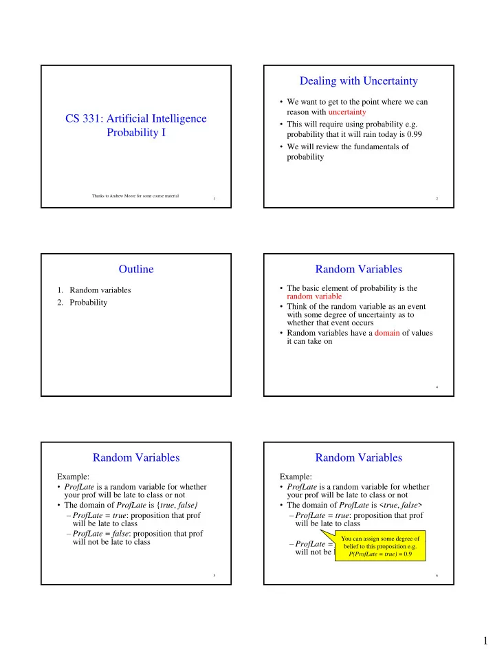
Dealing with Uncertainty • We want to get to the point where we can reason with uncertainty CS 331: Artificial Intelligence • This will require using probability e.g. Probability I probability that it will rain today is 0.99 • We will review the fundamentals of probability Thanks to Andrew Moore for some course material 1 2 Outline Random Variables • The basic element of probability is the 1. Random variables random variable 2. Probability • Think of the random variable as an event with some degree of uncertainty as to whether that event occurs • Random variables have a domain of values it can take on 4 Random Variables Random Variables Example: Example: • ProfLate is a random variable for whether • ProfLate is a random variable for whether your prof will be late to class or not your prof will be late to class or not • The domain of ProfLate is { true , false} • The domain of ProfLate is < true , false > – ProfLate = true : proposition that prof – ProfLate = true : proposition that prof will be late to class will be late to class – ProfLate = false : proposition that prof You can assign some degree of will not be late to class – ProfLate = false : proposition that prof belief to this proposition e.g. will not be late to class P(ProfLate = true) = 0.9 5 6 1

Random Variables Random Variables • We will refer to random variables with Example: capitalized names e.g. X , Y , ProfLate • ProfLate is a random variable for whether • We will refer to names of values with lower your prof will be late to class or not case names e.g. x , y , proflate • The domain of ProfLate is < true , false > • This means you may see a statement like – ProfLate = true : proposition that prof ProfLate = proflate will be late to class – This means the random variable ProfLate takes the value proflate (which can be true or false ) – ProfLate = false : proposition that prof • Shorthand notation : will not be late to class ProfLate = true is the same as proflate and And to this one e.g. ProfLate = false is the same as ¬ proflate P(ProfLate = false) = 0.1 7 8 Random Variables Boolean Random Variables • Take the values true or false 3 types of random variables: • E.g. Let A be a Boolean random variable 1. Boolean random variables – P(A = false) = 0.9 2. Discrete random variables – P(A = true) = 0.1 3. Continuous random variables 10 Discrete Random Variables Discrete Random Variables Values of the domain must be: Allowed to taken on a finite number of values • Mutually Exclusive i.e. P( A = v i AND A = v j ) = 0 e.g. if i  j • P(DrinkSize=small) = 0.1 This means, for instance, that you can’t have a • P(DrinkSize=medium) = 0.2 drink that is both small and medium • Exhaustive i.e. P(A = v 1 OR A = v 2 OR ... OR A = • P(DrinkSize=large) = 0.7 v k ) = 1 This means that a drink can only be either small , medium or large . There isn’t an extra large. 2

Discrete Random Variables Discrete Random Variables • Since we now have multi-valued discrete Values of the domain must be: • Mutually Exclusive i.e. P( A = v i AND A = v j ) = 0 random variables we can’t write P(a) or if i  j P(¬a) anymore This means, for instance, that you can’t have a The AND here means intersection • We have to write P(A = v i ) where v i = a i.e. (A = v i )  (A = v j ) drink that is both Small and Medium value in { v 1 , v 2 , …, v k } • Exhaustive i.e. P(A = v 1 OR A = v 2 OR ... OR A = v k ) = 1 This means that a drink can only be either small , The OR here means union i.e. (A = v 1 )  medium or large . There isn’t an extra large (A = v 2 )  ...  (A = v k ) 14 Probability Density Functions Continuous Random Variables Discrete random variables have probability distributions: • Can take values from the real numbers 1.0 • E.g. They can take values from [0, 1] P( A ) • Note: We will primarily be dealing with discrete random variables a ¬a Continuous random variables have probability density • (The next slide is just to provide a little bit functions e.g: of information about continuous random P( X ) P( X ) variables) X X 15 Probabilities Probabilities • We will sometimes talk about the • We will write P(A=true) as “the fraction of probabilities of all possible values of a possible worlds in which A is true” random variable • We can debate the philosophical • Instead of writing implications of this for the next 4 hours – P(A=false) = 0.25 • But we won’t – P(A=true) = 0.75 • We will write P ( A ) = (0.25, 0.75) Note the boldface! 18 3

Visualizing A The Axioms of Probability • 0  P( a )  1 • P( true ) = 1 • P( false ) = 0 Event space of all possible P( a ) = Area of Worlds in which • P( a OR b ) = P( a ) + P( b ) - P( a AND b ) worlds reddish oval A is true The logical OR is equivalent to set Its area is 1 The logical AND is equivalent to union  . Worlds in which A is false set intersection (  ). Sometimes, I’ll write it as P(a, b) These axioms are often called Kolmogorov’s axioms in honor of the Russian mathematician Andrei Kolmogorov 19 20 Interpreting the axioms Interpreting the axioms • 0  P( a )  = 1 • 0  P( a )  1 • • P( true ) = 1 P( true ) = 1 • P( false ) = 0 • P( false ) = 0 • • P( a OR b ) = P( a ) + P( b ) - P( a, b ) P( a OR b ) = P( a ) + P( b ) - P( a, b ) The area of P( a) can’t The area of P( a) can’t get any smaller than 0 get any bigger than 1 And a zero area would And an area of 1 would mean that there is no mean all worlds will have world in which a is not a is true false 21 22 Interpreting the axioms Prior Probability • 0  P( a )  1 • We can consider P(A) as the unconditional • P( true ) = 1 or prior probability • P( false ) = 0 • P( a OR b ) = P( a ) + P( b ) - P( a, b ) – E.g. P(ProfLate = true) = 1.0 P( a, b ) [The purple area] • It is the probability of event A in the absence of any other information • If we get new information that affects A , we a b can reason with the conditional probability of A given the new information. P( a OR b ) [the area of both circles] 23 24 4

Conditional Probability Conditional Probability Example • P( A | B ) = Fraction of worlds in which B is H = “Have a headache” F = “Coming down with true that also have A true F Flu” • Read this as: “Probability of A conditioned P( H ) = 1/10 on B ” P( F ) = 1/40 P( H | F ) = 1/2 • Prior probability P( A ) is a special case of the H “Headaches are rare and flu conditional probability P( A | ) conditioned on is rarer, but if you’re coming no evidence down with ‘flu there’s a 50 - 50 chance you’ll have a headache.” 25 26 Conditional Probability Definition of Conditional Probability P( H | F ) = Fraction of flu-inflicted ( , ) P A B F worlds in which you have a  ( | ) P A B headache ( ) P B # worlds with flu and headache  # worlds with flu H Area of " H and F" region Corollary: The Chain Rule (aka The Product Rule)  Area of " F" region  P(H, F)  ( , ) ( | ) ( ) P A B P A B P B H = “Have a headache” P(F) F = “Coming down with Flu” P( H ) = 1/10 P( F ) = 1/40 27 28 P( H | F ) = 1/2 Important Note The Joint Probability Distribution    • P( A , B ) is called the joint probability ( | ) ( | ) 1 P A B P A B distribution of A and B • It captures the probabilities of all But: combinations of the values of a set of    random variables ( | ) ( | ) does not always 1 P A B P A B 29 30 5

The Joint Probability Distribution The Joint Probability Distribution • Now suppose we have the random variables: • For example, if A and B are Boolean – Drink = { coke , sprite } random variables, then P( A , B ) could be – Size = { small , medium, large } specified as: • The joint probability distribution for P( Drink , Size ) could look like: P( A = false , B = false ) 0.25 P( A = false , B = true ) 0.25 P( Drink = coke , Size = small ) 0.1 P( A = true , B = false ) 0.25 P( Drink = coke , Size = medium ) 0.1 P( A = true , B = true ) 0.25 P( Drink = coke , Size = large ) 0.3 P( Drink = sprite , Size = small ) 0.1 P( Drink = sprite , Size = medium ) 0.2 P( Drink = sprite , Size = large ) 0.2 31 32 Full Joint Probability Distribution • Suppose you have the complete set of random variables used to describe the world • A joint probability distribution that covers this complete set is called the full joint probability distribution • Is a complete specification of one’s uncertainty about the world in question • Very powerful: Can be used to answer any probabilistic query 33 6