DARK ENERGY PROBES Phenomenology Enrique Gaztaaga, ICE (IEEC/CSIC) - - PowerPoint PPT Presentation

1

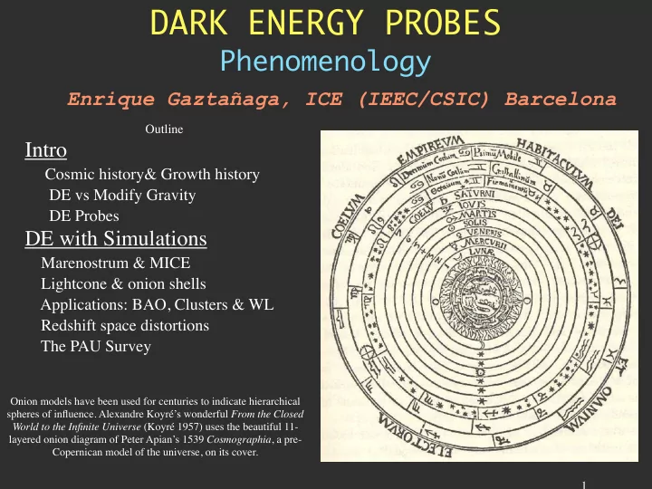
Onion models have been used for centuries to indicate hierarchical spheres of influence. Alexandre Koyré’s wonderful From the Closed World to the Infinite Universe (Koyré 1957) uses the beautiful 11- layered onion diagram of Peter Apian’s 1539 Cosmographia, a pre- Copernican model of the universe, on its cover.

Outline

Intro

Cosmic history& Growth history DE vs Modify Gravity DE Probes

DE with Simulations

Marenostrum & MICE Lightcone & onion shells Applications: BAO, Clusters & WL Redshift space distortions The PAU Survey

DARK ENERGY PROBES

Phenomenology

Enrique Gaztañaga, ICE (IEEC/CSIC) Barcelona

Two driving questions in Cosmology:

Background: Evolution of scale a(t)

+ Symmetries + Einstein’s Eq. (Gravity?) + matter-energy content ?

• > Friedman Eq.:

H2(z) = H2

0 [ ΩM (1+z)3 + ΩR (1+z)4 +

ΩK(1+z)2 + ΩDE (1+z)3(1+w) ] c dt = a dχ -> χ = c ∫dz/H(z) Dark Matter and Dark Energy!

Structure Formation:

+ origin of structure (Initial Conditions) + gravitational instability (Gravity?) + matter-energy content ?

δL’’ + H δL’ - 3/2 Wm H2 δL = 0

+ galaxy/star formation (SFR): bias

HOW DID WE GET HERE?

3

Observables

H(z) = cΔzBAO π BAO dA(z) = σ BAO ΔθBAO

(Angular) Comoving distance Comoving Radial distance

cdt = adr => cdz = Hπ

Observer

dA θ σ

π = c H(z) dz Sk(χ)−1 ≡ dA(z) = cdz′′ H(z′)

z

∫

= (1+ z)DA(z)

π

M = m + 2.5 log(dL/ 10pc) dL= dA (1+z)= DA (1+z)2

Luminosity distance Comoving Horizon scale = conformal time

t = cda aH

a

∫

Age

η ≡ χ H = cdt a

t

∫

= cda a2H

a

∫

(null) Light-like radial (dΩ=0) events

Comoving transverse separation σ = dAθ Comoving radial separation π = cdz/H

z1 z2 dz= z2 - z1 - r2 = σ2 + π2 π ≡ dr Light-like angular (dr=0) events cdt = a rθ

Observed Known

Using galaxies to trace structure Alcock-Paczynski (1979) test

Where does Structure in the Universe come From? How did galaxies/star/molecular clouds form?

time Initial

• verdensed

seed background Overdensed region Collapsed region = DM hierarchical halos

Stage-I: gravitational collapse from some initial seeds

Physical scales

Stage-II: baryon radiative cooling into gas and stars

H2 dust

STARS

DM remains In halos

Disk formation: colapse is faster in direction parallel to spin axis

VIRGO N-body simulations

Mass conservation Euler Eq. dτ =a dt

Jeans Instability (linear regime)

δL(x,τ) = D(τ) δ0(x) EdS Λ Open

a = 1/(1+z)

z = 0 (now) z = 9

Another handle on DE:

• Where Friedman Eq. (Expansion history) may not

separate modified gravity from DE: Growth of sctructure could: models with equal expansion history yield difference D(z) (EG & Lobo

2001), astro-ph/0303526 & 0307034)

δ

• = D
• Dδ = −

r ∇ r v a ≡ −Hθ

θ = − f(Ω) δ

Velocity growth factor: tell us if gravity is really responsible for structure! Could also tell us about cosmological parameters EdS

Weakly non-linear Perturbation Theory

EdS

MODE COUPLING

k1 k2 µ=cosθ

3 1 2

k12

Linear Theory: modes are independent

2nd order containts mode couplings Coupling functions:

• adimensional
• geometrical
• Non-linear
• Gravitational instability

Observations require an statistical approach:

Evolution of (rms) variance ξ2 = < δ2> instead of δ Or power spectrum P(k)= < δ2(k)> => ξ2 = ∫ dk P(k) k2 W(k) dk

IC problem: Linear Theory δ = D δ0 ξ2 = < δ2> = D2 < δ0

2>

Normalization σ8 2 ≡ < δ2(R=8)> To find D(z) -> Compare < δ2> at two times or find evolution invariants

Problem: statistical bias: δgal = b δdm => < δ2

gal> = b2 < δ2 dm>

So linear measurements constrain degenerate product: D(z)*b(z) ; b*σ8

θ = − f(Ω) δ = − f(Ω)/b δgal β

Initial Gaussian distribution of density fluctuations: ξp (V) = < δP>c = 0 for all p ≠2 Perturbations due to gravity generate non-zero ξp

−> ξ3 = S3 ξ2

2 with S3(m)= 34/7 (time invariant)

11

Bias: lets take a very simple model. rare peaks in a Gaussian field (Kaiser 1984, BBKS)

Linear bias “b”: δ (peak) = b δ(mass) with b= ν/σ (SC: ν=δc/σ)

−> ξ2 (peak) = b2 ξ2 (m)

Threshold ν

Local bias

δh= F[ δm] =

b δm + b2 δm

2

c 2 ≡ b2 / b

Does light traces mass?

14

What is Dark Energy?

MG is degenerate with DE if we only use Cosmic history: need Growth history:

Lue, Scoccimarro & Starkman astro-ph/0307034 working examples: Brans-Dicke, f(R), DGP

ds2= - [1+ 2 Ψ(t,x) ] dt2 + a2 [1-2 ϕ(t,x)] dr2 -k2 ϕ(a,k) = 4π a2 G g(k) ρ δ

η ≡ Curvature ϕ /Newtonian Ψ effective G g(k) Mukhanov, Feldman & Branderberger (1992)

1 Whatever Energy-Momemtum Tensor is needed in Einstein Field Eq. (assumes GR)

Guzik, Jain & Takada 2009 arXiv:0906.2221

2 Whatever causes cosmic acceleration includes Modified Gravity(MG)

General Relativity vs Brans-DicKe

a(t) = scale factor =1/(1+z) (a_0 = 1 ) Einstein's Field Eq. R = curvature/metric T = matter content

Hubble Cte (Friedman Eq)

Flux= L/4πDL

2

ω > 2500 (solar system) δ = δ0 a (1+ω)/(2 +ω)

EG & A.Lobo astro-ph/0003129, ApJ, v548, 47-59, 2001

• T. Damour & K. Nortdvedt, Phys. Rev. D 48, 3436 (1993)

B.~Boisseau, G.~Esposito-Far\`ese, D.~Polarski, and A.A.~Starobinsky, Phys. Rev. D, 59, 123502, 1999 S.~Sen and A.A.~Sen,Phys. Rev. D in press 2001 (gr-qc/0010092)

DES= Dark Energy Survey

• Study Dark Energy using

4 complementary* techniques:

• I. Cluster Counts
• II. Weak Lensing
• III. Baryon Acoustic Oscillations
• IV. Supernovae
• Two multiband surveys:

5000 deg2 g, r, i, Z,Y to i~24

9 deg2 repeat (SNe)

• Build new 3 deg2 camera

and Data management system

Survey 30% of 5 years Response to NOAO AO DES Forecast: FoM =4.6x

*in systematics & in cosmological parameter degeneracies *geometric+structure growth: test Dark Energy vs. Gravity

Photometric Redshifts

• Measure relative flux in

multiple filters: track the 4000 A break

• Estimate individual galaxy

redshifts with accuracy σ(z) < 0.1 (~0.02 for clusters)

• Precision is sufficient

for Dark Energy probes, provided error distributions well measured.

• Good detector response

in z band filter needed to reach z>1 Elliptical galaxy spectrum

• I. Clusters and Dark Energy
• Requirements

1.Understand formation of dark matter halos 2.Cleanly select massive dark matter halos (galaxy clusters)

• ver a range of redshifts

3.Redshift estimates for each cluster 4.Observable proxy that can be used as cluster mass estimate: g(O|M,z) Primary systematics: Uncertainty in g (bias & scatter) Uncertainty in O selection fn.

dN(z) dzdΩ = dV dz dΩ n z

( )

Number of Clusters vs. Redshift w = −1 w = −1

Observer Dark matter halos Background sources



Statistical measure of shear pattern, ~1% distortion



Radial distances depend on geometry of Universe



Foreground mass distribution depends on growth of structure

• II. Weak Lensing: Cosmic Shear
• Cosmic Shear Angular Power Spectrum in

Photo-z Slices

• Shapes of ~300 million well-resolved

galaxies, 〈z〉 = 0.7

• Primary Systematics:

photo-z’s, PSF anisotropy, shear calibration

• Extra info in bispectrum & galaxy-shear:

robust

• III. Baryon Acoustic Oscillations

CMB Angular Power Spectrum

SDSS galaxy correlation function Acoustic series in P(k) becomes a single peak in ξ(r) Bennett, etal Eisenstein etal

• IV. Supernovae
• Geometric Probe of Dark Energy
• Baseline: repeat observations of 9 deg2 using

10% of survey time: 5 visits per lunation in riz

• ~1100-1400 well-measured SN Ia

lightcurves to z~1

• Larger sample, improved z-band response

(fully depleted CCDs) compared to ESSENCE, SNLS: reduce dependence on rest-frame u-band and Malmquist bias

• Spectroscopic follow-up of large SN

subsample+host galaxies (LBT, Magellan, Gemini, Keck, VLT,…) e.g., focus on ellipticals (low dust extinction) SDSS

DES Forecasts: Power of Multiple Techniques

Assumptions: Clusters: σ8=0.75, zmax=1.5, WL mass calibration (no clustering) BAO: lmax=300 WL: lmax=1000 (no bispectrum) Statistical+photo-z systematic errors only Spatial curvature, galaxy bias marginalized, Planck CMB prior Factor 4.6 improvement over Stage II w(z) =w0+wa(1–a) 68% CL

geometric geometric+ growth

DETF Figure of Merit: inverse area of ellipse Stage II not included here

PRIMARY & SECONDARY CMB ANISOTROPIES

Sachs-Wolfe (ApJ, 1967)

ΔT/T(n) = [ 1/4 δγ (n) + v.n + Φ (n) ]i

f

• Temp. F. = Photon-baryon fluid AP + Doppler + N.Potential (SW)

Φi Φf

In EdS: D(z) = a, so that Φ ~δM/R~ D/a~cte and therefore ΔT/T = dΦ/dτ = 0 In DE universe => < ΔT/T δG> ≠ 0

+ Integrated Sachs-Wolfe (ISW) & Rees-Sciama (Nature, 1968) non-linear

2 ∫if dτ dΦ/dτ (n)

EG, Manera, Multamaki (astro-ph/ 0407022)

DARK ENERGY PROBES

PROBE Photometric Survey Spectroscopic Survey (z<1) Spectroscopic Follow-up

CMB

SNe-Ia X X BAO Y Y X WL X

z-distortions

X

clusters

X Y X Y ISW X X Y = OPTIONAL X = REQUIRED

Padmanabhan

25

Tools for precision DE Test

1. BAO oscilations in galaxies 2. Redshift space distortions 3. Weak gravitational lensing 4. Galaxy Cluster count 5. SNIa

New Challenges

1. Systematic (calibration, bias) 2. Separate Galaxy from Cosmic Evolution 3. Accurate errors 4. New theoretical models

New Surveys

DES: Dark Energy Survey PanStars, LSST... SDSS3 (BOSS), PAU

NEXT GENERATION SIMULATIONS:

MICE

project web: www.ice.cat/mice

Project to develop very large numerical simulations in cosmology using the Marenostrum supercomputer (Barcelona)  10.000 processors, 20 TB RAM , 100 Teraflops  GADGET N-body simulations with 109-1010 dark-matter particles in volumes 1-500 Gpc3 ï dynamical range of 5 orders of magnitude  Terabytes of simulated data stored at Port d’Informació Cientifica (LHC data storage center @ Barcelona) ➣Team: (core@ICE): P.Fosalba, F.Castander,E.Gaztañaga Collaborators: V.Springel (MPA), C.Baugh (Durham), M.Manera (NYU), M.Crocce, A.Gonzalez, A.Cabré,

Where do we stand ?

Millennium (Springel et al 2006)

N Box Mass

10243 1500 Mpc 2.4 1011 Msun 10243 3000 Mpc 1.9 1012 Msun 20483 3000 Mpc 2.4 1011 Msun 20483 7700 Mpc 3.7 1012 Msun 40963 3000 Mpc 3.0 1010 Msun runing….

Millennium Simulation:

21603 500 Mpc 9 108 Msun

Volume MICE ~ 200x Millennium Resotucion MICE ~ 64x Hubble Vol BAO scale to 1% accuracy

“Onion shells”

• bserver

(P.Fosalba et al, arXiv:0711.1540)

Angular Spectrum For single redshift slice: z =0.9-1.0 Of MICE Simulation

www.ice.cat/mice

Turnover

Baryon wiggles

30

Convergence Maps

31

Cosmos

Convergence Maps Sampling Variance

(P.Fosalba et al, arXiv:0711.1540)

32

Text

• Mass function is not universal
• Excess of VERY massive halos
• 50% bias in DE parameters

Text

Crocce etal 2009 astro-ph/0907.0019

θ = − β δ

Real Space Redshift Space

Large Small scales scales

redshift space distortions

34

R a d i a l π Transverse σ

Real Space Redshift Space

θ = − β δ

Observer

vp= π−σ

Anna Cabré’s PhD Thesis arXiv:0807.3551

Large scales Small scales Growth mass

2-point Correlation

≡ < δ(r1) δ(r2) >

35

Anna Cabré’s PhD Thesis arXiv:0807.3551

Errors from MICE sim

Radial BAO: shape method

Gaussian priors: ΩB = 0.044± 0.003 (WMAP5) Ωm = 0.245± 0.020 (paper-I) β = 0.34± 0.03 (paper-I) b*σ8 = 1.56 ± 0.09 (paper-I) Flat Priors: A = 2 ± 3 (lensing mag.)

h=0.72, n=0.96, σ8 =0.85

H(z=0.34)= 83.9 ± 3.1 (± 0.8) Km/s (h/0.72)

Does not need a standard ruler

Summary Radial BAO

• Radial correlation matches well model:
• 3.2σ detection of BAO, 2σdection of lensing
• Measurements of H(z) with 2 methods:

– Shape in 40-140 Mpc/h range (marginalized):

• H(z=0.34)= 83.87 ± 3.10 (± 0.84) Km/s/Mpc (h/0.72)

– Peak location between 100-120 Mpc/h (+BAO-WMAP5):

• H(z=0.24)= 79.69 ± 2.32 (± 1.29) km/s/Mpc
• H(z=0.34)= 83.80 ± 2.96 (± 1.59) Km/s/Mpc (not independent)
• H(z=0.43)= 86.45 ± 3.27 (± 1.69) Km/s/Mpc

37 arXiv:0808.1921

CAN THIS BE IMPROVED?

Requirements on Redshift Precision

Δz / (1+z) Δz / (1+z)

H(z) dA(z)

PAU PAU

spec spec photo photo

Inverse of area of w0-wa error ellipse Padmanabhan

38

Spectroscopic accuracy is not needed: trade-off with number density

Can Many Narrow Filters Do The Trick? PAU Survey

39 We explore the performance of a photometric system with 40 medium band non-overlaping filters (100A width)similar to that of ALHAMBRA but with more and narrower filters.

Redshift Resolution

LRGs with L>L* mI<23

40

BAO LRG survey in a 2m (effective) class telescope (Ef.Etendue ~20) with a ~6 deg2 FoV camera equipped with ~40 10nm-wide filters, ~500 Mpixels with 0.35”/pixel.

• 8,000 deg2 in 4 years (but we have dedicated use of

telescope for 5 years)

• 0.1 < z < 0.9
• mI < 23
• nLRG > 10-3 (h/Mpc)3, nP ~10 at all scales
• V ~ 25 Gpc3 ~ 9 (Gpc/h)3
• NLRG ~ 14 million (L > L*, iAB < 22.5)
• Ngalaxy ~ 200 million

PAU-BAO Survey

41

Selection effects

The Astrophysical Journal, V691,241-260 (2009) arXiv:0807.0535

DARK ENERGY PROBES

PROBE Photometric Survey Spectroscopic Survey (z<1) Spectroscopic Follow-up

CMB

SNe-Ia X X BAO Y Y X WL X

z-distortions

X

clusters

X Y X Y ISW X X Y = OPTIONAL X = REQUIRED

Padmanabhan