
SLIDE 1
D T E
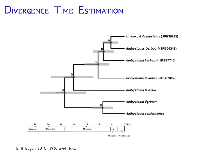
Bi & Bogart 2010. BMC Evol. Biol.
D T E Bi & Bogart 2010. BMC - - PowerPoint PPT Presentation
D T E Bi & Bogart 2010. BMC Evol. Biol. D T E Methods estimate the SUBSTITUTION RATE and TIME separately Branch
Bi & Bogart 2010. BMC Evol. Biol.
Branch lengths = SUUBSTITION RATE X TIME Branch lengths = SUBSTITUTION RATE Branch lengths = TIME
◮ Global molecular clock (Zuckerkandl & Pauling, 1962) ◮ Local molecular clocks (Kishino, 1990; Rambaut & Bromham
◮ Compound Poisson process (Huelsenbeck et al., 2000) ◮ Autocorrelated rates – Log-normal distribution (Thorne et al.,
◮ Uncorrelated rates (Drummond et al., 2006, Rannala &
◮ Non-parametric rate smoothing/Penalized likelihood
◮ Ornstein-Uhlenbeck Process (Aris-Brosou & Yang, 2002) ◮ Cox–Ingersol–Ross process (Lepage et al., 2006)
Branch lengths = SUUBSTITION RATE X TIME Branch lengths = SUBSTITUTION RATE Branch lengths = TIME
(Zuckerkandl & Pauling, 1962)
◮ Almost any error in the
◮ Assumption of a Poisson
Branch lengths = SUUBSTITION RATE X TIME Branch lengths = SUBSTITUTION RATE Branch lengths = TIME
◮ mutation rates can vary
◮ strength and targets of
◮ population sizes can
Branch lengths = SUUBSTITION RATE X TIME Branch lengths = SUBSTITUTION RATE Branch lengths = TIME
low high rate
(Kishino, 1990; Rambaut & Bromham 1998; Yang & Yoder, 2003)
low high rate
(Huelsenbeck et al., 2000)
low high rate
(Thorne et al., 1998; Kishino & Thorne, 2001; Thorne et al., 2002)
low high rate
(Drummond et al., 2006)
cave bear American black bear sloth bear Asian black bear brown bear polar bear American giant short-faced bear giant panda sun bear harbor seal spectacled bear 4.08 5.39 5.66 12.86 2.75 5.05 19.09 35.7 0.88 4.58
[3.11–5.27] [4.26–7.34] [9.77–16.58] [3.9–6.48] [0.66–1.17] [4.2–6.86] [2.1–3.57] [14.38–24.79] [3.51–5.89] 14.32 [9.77–16.58] 95% CI mean age (Ma)t 2 t 3 t 4 t 6 t 7 t 5 t 8 t 9 t 10 t x
node MP•MLu•MLp•Bayesian 100•100•100•1.00 100•100•100•1.00 85•93•93•1.00 76•94•97•1.00 99•97•94•1.00 100•100•100•1.00 100•100•100•1.00 100•100•100•1.00t 1 Eocene Oligocene Miocene Plio Plei Hol 34 5.3 1.8 23.8 0.01 Epochs Ma
Global expansion of C4 biomass Major temperature drop and increasing seasonality Faunal turnoverKrause et al., 2008. Mitochondrial genomes reveal an explosive radiation of extinct and extant bears near the Miocene-Pliocene boundary. BMC Evol. Biol. 8.
Taxa 1 5 10 50 100 500 1000 5000 10000 20000 100 200 300 MYA Ophidiiformes Percomorpha Beryciformes Lampriformes Zeiforms Polymixiiformes
Aulopiformes Myctophiformes Argentiniformes Stomiiformes Osmeriformes Galaxiiformes Salmoniformes Esociformes Characiformes Siluriformes Gymnotiformes Cypriniformes Gonorynchiformes Denticipidae Clupeomorpha Osteoglossomorpha Elopomorpha Holostei Chondrostei Polypteriformes Clade r ε "AIC 1. 0.041 0.0017 25.3 2. 0.081 * 25.5 3. 0.067 0.37 45.1 4. * 3.1 Bg. 0.011 0.0011
Acanthomorpha Teleostei
ray-finned fishes. BMC Evol. Biol. 9.
Uniform prior Birth-death prior
Lepage et al., 2007. A General Comparison of Relaxed Molecular Clock Models. MBE 24:2669–2680.
Time
Time
fossil age present
(Benton & Donoghue 2007 Mol. Biol. Evol. 24(1):26–53)
(Benton & Donoghue 2007 Mol. Biol. Evol. 24(1):26–53)
(Benton & Donoghue 2007 Mol. Biol. Evol. 24(1):26–53)
(Benton & Donoghue 2007 Mol. Biol. Evol. 24(1):26–53)
Uniform ( , ? )
Time
fossil age present
Exponential (λ) Gamma (α, β) Uniform ( , ∞)
Time
fossil age present
Time
◮ Dependent on and sensitive to fossil calibrations – fossil
◮ Models are not biologically realistic ◮ Different methods/models can produce very different
◮ Priors are too informative ◮ Studies comparing methods have produced conflicting
(Butler, 2007 Nature)
(de Oliveria et al., 2006 Nature)
(de Oliveria et al., 2006 Nature)