Curves and paths in space Example : Define ( t ) := (cos t, sin t ) - - PowerPoint PPT Presentation

Curves and paths in space

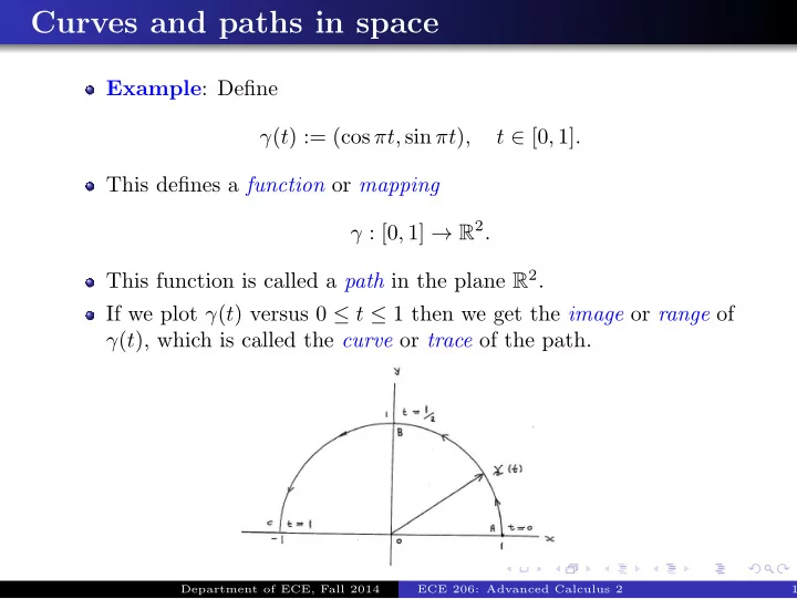
Example: Define γ(t) := (cos πt, sin πt), t ∈ [0, 1]. This defines a function or mapping γ : [0, 1] → R2. This function is called a path in the plane R2. If we plot γ(t) versus 0 ≤ t ≤ 1 then we get the image or range of γ(t), which is called the curve or trace of the path.

Department of ECE, Fall 2014 ECE 206: Advanced Calculus 2 1/18

Parametric representation of curves

Definition A two-dimensional path (or parametric function for a two-dimensional curve) is a given function or mapping γ : [0, 1] → R2, from a specified interval [a, b] into R2, which maps each a ≤ t ≤ b into the vector γ(t) ∈ R2. In terms of scalar components, we usually write: γ(t) = (x(t), y(t)) = x(t)i + y(t)j, ∀t ∈ [a, b]. The curve of the path is the set of points Γ ⊂ R2 traced by γ(t) as t traverses the interval [a, b]. Formally: Γ :=

• γ(t) ∈ R2 | t ∈ [a, b]
• .

Department of ECE, Fall 2014 ECE 206: Advanced Calculus 2 2/18

Parametric representation of curves (cont.)

The interval a ≤ t ≤ b is called the parametric interval, t is called the parametric variable of the path, and the whole function γ(t) is called a parametric representation of the curve Γ. The starting point of the path is the vector γ(a), while the ending point of the path is the vector γ(b). The curve Γ has a direction from the starting to the ending point corresponding to t increasing from t = a until t = b.

Department of ECE, Fall 2014 ECE 206: Advanced Calculus 2 3/18

Parametric curves in R3

Definition A three-dimensional path (or parametric function for a three-dimen- sional curve) is a given function or mapping γ : [0, 1] → R3, from a specified interval [a, b] into R3, which maps each a ≤ t ≤ b into the vector γ(t) ∈ R3. Usually, γ(t) is written in the scalar component form γ(t) = (x(t), y(t), z(t)) = x(t)i + y(t)j + z(t)k, ∀t ∈ [a, b]. The curve of the path is the set of points Γ ⊂ R3 traced by γ(t) as t traverses the interval a ≤ t ≤ b. Formally: Γ :=

• γ(t) ∈ R3 | t ∈ [a, b]
• .

Department of ECE, Fall 2014 ECE 206: Advanced Calculus 2 4/18

Parametric curves in R3 (cont.)

The remaining definitions are word-for-word identical to the R2 case, except that everywhere we just replace R2 with R3.

Department of ECE, Fall 2014 ECE 206: Advanced Calculus 2 5/18

More definitions

Definition If the path γ : [a, b] → R3 is such that the first derivatives dx(t) dt , dy(t) dt , dz(t) dt exist and are continuous for each t ∈ [a, b], then γ is called a C1-path and the curve corresponding to γ is called a C1-curve. Definition If γ : [a, b] → R3 is a C1 path and additionally the derivatives d2x(t) dt2 , d2y(t) dt2 , d2z(t) dt2 exist and are continuous for each t ∈ [a, b], then γ is called a C2-path and the curve corresponding to γ is called a C2-curve.

Department of ECE, Fall 2014 ECE 206: Advanced Calculus 2 6/18

Paths and curves

Different paths can have identical curves! For example, define γ(t) := (cos(2πt), sin(2πt)), 0 ≤ t ≤ 1/2, which results in a mapping γ : [0, 1/2] → R2. The curve corresponding to this path is identical to that of (cos πt, sin πt) with t ∈ [0, 1].

Department of ECE, Fall 2014 ECE 206: Advanced Calculus 2 7/18

Paths and curves (cont.)

To further illustrate the idea, let us define γ1(t) = (cos πt, sin πt) with t ∈ [0, 1]. Now define the function ψ : [1, √ 2] → R, ψ(s) := s2 − 1. We see that ψ(1) = 0, ψ( √ 2) = 1, ψ′(s) = 2s > 0, ∀s ∈ [1, √ 2]. The function ψ(s) increases strictly monotonically through the interval [0, 1] as s increases through the interval 1 ≤ s ≤ √ 2.

Department of ECE, Fall 2014 ECE 206: Advanced Calculus 2 8/18

Paths and curves (cont.)

Now define the path γ2 : [1, √ 2] → R2 as γ2(s) := γ1(ψ(s)) =

• cos(π(s2 − 1)), sin(π(s2 − 1))
• , 1 ≤ s ≤
• (2).

The paths γ1 and γ2 are clearly different, but they nevertheless have the same curve. In fact, γ1 and γ2 are distinct parametric representations of the same curve.

Department of ECE, Fall 2014 ECE 206: Advanced Calculus 2 9/18

Re-parametrization

More generally, suppose we have γ1 : [a1, b1] → R3. In order to change the parametrization to get a different path with exactly the same curve, we fix some interval [a2, b2] along with some strictly increasing C1-function ψ : [a2, b2] → R such that ψ(a2) = a1, ψ(b2) = b1, ψ′(s) > 0, ∀s ∈ [a2, b2]. Then the path γ2 : [a2, b2] → R3 defined by γ2(s) := γ1(ψ(s)), a2 ≤ s ≤ b2 gives a different parametric representation of the same curve.

Department of ECE, Fall 2014 ECE 206: Advanced Calculus 2 10/18

Tangent to a curve

Given a path γ : [a, b] → R3 represented as γ(t) = (x(t), y(t), z(t)) = x(t)i + y(t)j + z(t)k, its derivative w.r.t t is the vector in R3 given by γ(1)(t) := dγ(t) dt = dx(t) dt , dy(t) dt , dz(t) dt

• = dx(t)

dt i+dy(t) dt j+dz(t) dt k, for all a ≤ t ≤ b. Similarly, the second derivative of the path w.r.t. t is given by γ(2)(t) := dγ(1)(t) dt = dx2(t) dt2 , dy2(t) dt2 , dz2(t) dt2

• =

= dx2(t) dt2 i + dy2(t) dt2 j + dz2(t) dt2 k, for all a ≤ t ≤ b.

Department of ECE, Fall 2014 ECE 206: Advanced Calculus 2 11/18

Tangent to a curve (cont.)

The fact that γ(t) = (x(t), y(t), z(t) along with dx dt = lim

∆t→0

x(t + ∆t) − x(t) ∆t dy dt = lim

∆t→0

y(t + ∆t) − y(t) ∆t dz dt = lim

∆t→0

z(t + ∆t) − z(t) ∆t suggests that dγ dt = lim

∆t→0

γ(t + ∆t) − γ(t) ∆t

Department of ECE, Fall 2014 ECE 206: Advanced Calculus 2 12/18

Tangent to a curve (cont.)

The difference vector γ(t + ∆t) − γ(t) is vey close to tangential to the curve of the path. When ∆t is small, and the limit of (γ(t + ∆t) − γ(t)) /∆t is exactly tangent to the curve of the path at γ(t). Thus, the derivative γ(1)(t) is tangent to the curve of the path γ : [a, b] → R3 at γ(t) for each instant a ≤ t ≤ b. Similarly, one can see that the derivative γ(2)(t) is tangent to the curve of the path γ(1) : [a, b] → R3 at γ(1)(t) for each a ≤ t ≤ b.

Department of ECE, Fall 2014 ECE 206: Advanced Calculus 2 13/18

Products of curves

Given two paths γ1 : [a, b] → R3 and γ2 : [a, b] → R3, the inner product of the vectors γ1(t) and γ2(t) in R3 for each a ≤ t ≤ b gives a scalar-valued function ϕ(t) := γ1(t) · γ2(t), a ≤ t ≤ b. By the rule for differentiation of products, we have: dϕ(t) dt = γ1(t) · γ(1)

2 (t) + γ1(t)(1) · γ2(t),

∀t ∈ [a, b].

Department of ECE, Fall 2014 ECE 206: Advanced Calculus 2 14/18

Velocity and acceleration

The parametric variable for a given path γ : [a, b] → R3 does not have any “physical” interpretation, in general. However, in many applications, t may be interpreted as time (and hence [a, b] as a time interval). Moreover, if γ(t) represents a physical point moving in space, one can introduce the notions of velocity v and acceleration a, namely v(t) := γ(1)(t), a(t) := γ(2)(t), for all a ≤ t ≤ b.

Department of ECE, Fall 2014 ECE 206: Advanced Calculus 2 15/18

Velocity and acceleration (cont.)

Now, let F : D → R3 be a vector field (e.g., a force acting on a particle of mass m) defined over the domain D ⊂ R3. Suppose that, in response to this force, the particle follows the path γ : [a, b] → R3. Newton’s second law then says that ma(t) = F(γ(t)), t ∈ [a, b]. Alternatively, one has mγ(2)(t) = F(γ(t)), t ∈ [a, b]. This is a second order vector differential equation which can, in principle, be solved to get the path γ : [a, b] → R3 followed by the particle if one knows the force vector field F.

Department of ECE, Fall 2014 ECE 206: Advanced Calculus 2 16/18

Simple curves and closed curves

Definition If the path γ : [a, b] → R3 has the property that, for any t1, t2 ∈ [a, b], γ(t1) = γ(t2) when t1 = t2, the corresponding curve is called simple. Simply put, a simple curve has the property that it does not “cross itself” anywhere (as opposed to non-simple curves).

Department of ECE, Fall 2014 ECE 206: Advanced Calculus 2 17/18

Simple curves and closed curves (cont.)

Definition If the path γ : [a, b] → R3 has the property that γ(a) = γ(b), the corresponding curve (simple or not) is called closed. A closed curve which is also simple is called a simple closed curve whereas a closed curve which does cross itself somewhere is a non- simple closed curve.

Department of ECE, Fall 2014 ECE 206: Advanced Calculus 2 18/18