
1
Scheduling & Synthesis of Control Programs
- p
t i m a l
w Gerd Behrman, Ed Brinksma, Ansgar Fehnker, Thomas Hune, Paul Pettersson, Judi Romijn, Frits Vaandrager, Henning Dierks
…, HSCC’01, TACAS’01, CAV’01, AIPS’02,….
C CUPPAAL UPPAAL
AMETIST
2
UC UCb b
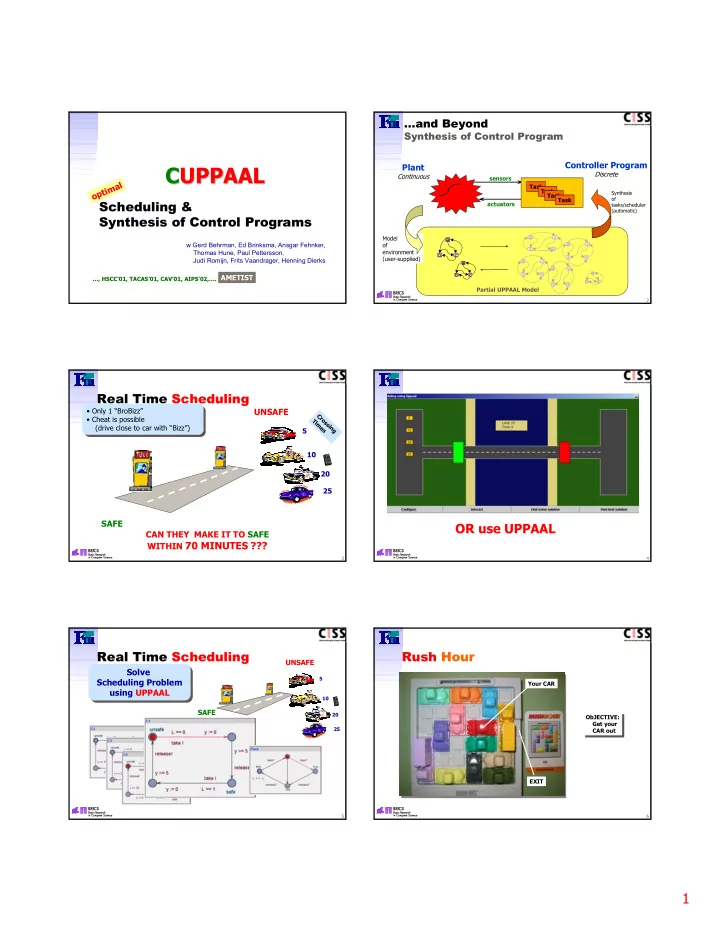
…and Beyond
Synthesis of Control Program
Plant
Continuous
Controller Program
Discrete
sensors actuators
a c b 1 2 4 3 a c b 1 2 4 3 1 2 4 3 1 2 4 3 a c b
Partial UPPAAL Model Model
- f
environment (user-supplied)
Synthesis
- f
tasks/scheduler (automatic)
Task Task Task Task
3
UC UCb b
Real Time Scheduling
5 10 20 25
UNSAFE SAFE
- Only 1 “BroBizz”
- Cheat is possible
(drive close to car with “Bizz”)
- Only 1 “BroBizz”
- Cheat is possible
(drive close to car with “Bizz”)
The Car & Bridge Problem CAN THEY MAKE IT TO SAFE WITHIN 70 MINUTES ???
Crossing Times
4
UC UCb b
Real Time Scheduling
5 10 20 25
UNSAFE
Give it a try on next lap-top !
- Only 1 “BroBizz”
- Cheat is possible
(drive close to car with “BroBizz”)
- Only 1 “BroBizz”
- Cheat is possible
(drive close to car with “BroBizz”)
OR use UPPAAL
5
UC UCb b
Real Time Scheduling
SAFE
5 10 20 25
UNSAFE
Solve Scheduling Problem using UPPAAL Solve Scheduling Problem using UPPAAL
6
UC UCb b
Rush Hour
ObJECTIVE: Get your CAR out ObJECTIVE: Get your CAR out Your CAR EXIT