CSE775: Computer Architecture Chapter 1: Fundamentals of Computer - - PDF document

1

CSE775: Computer Architecture

1

Chapter 1: Fundamentals of Computer Design

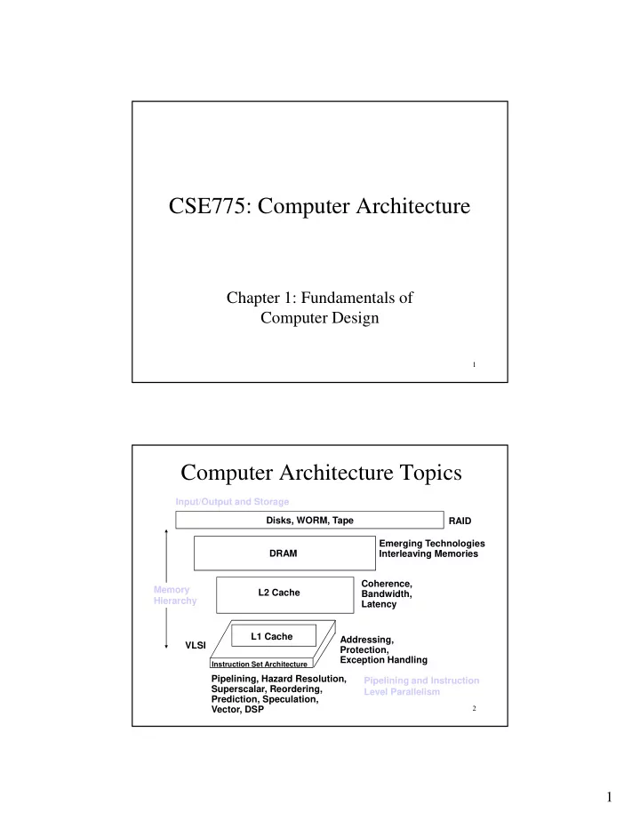
Computer Architecture Topics

Disks, WORM, Tape RAID Input/Output and Storage C L2 Cache DRAM Coherence, Bandwidth, Latency Emerging Technologies Interleaving Memories Memory Hierarchy

2 Instruction Set Architecture

Pipelining, Hazard Resolution, Superscalar, Reordering, Prediction, Speculation, Vector, DSP Addressing, Protection, Exception Handling L1 Cache VLSI Pipelining and Instruction Level Parallelism

2

Computer Architecture Topics

M P M P M P M P

Shared Memory, Message Passing,

M Interconnection Network S P M P M P M P ° ° °

Topologies, Routing, Bandwidth Network Interfaces g g, Data Parallelism

Processor-Memory-Switch

Multiprocessors

3

Bandwidth, Latency, Reliability Multiprocessors Networks and Interconnections

Measurement and Evaluation

Design

Architecture is an iterative process:

• Searching the space of possible designs
• At all levels of computer systems

Analysis

Creativity

Cost / Performance

4

Good Ideas Good Ideas

Mediocre Ideas

Bad Ideas

Performance Analysis

3

Issues for a Computer Designer

• Functional Requirements Analysis (Target)

– Scientific Computing – High Performance Floating pt. – Business – transactional support/decimal arithmetic Business transactional support/decimal arithmetic – General Purpose –balanced performance for a range of tasks

• Level of software compatibility

– PL level

• Flexible, Need new compiler, portability an issue

– Binary level (x86 architecture)

5

– Binary level (x86 architecture)

• Little flexibility, Portability requirements minimal
• OS requirements

– Address space issues, memory management, protection

• Conformance to Standards

– Languages, OS, Networks, I/O, IEEE floating pt.

Computer Systems: Technology Trends

• 1988
• 2008
• 1988

– Supercomputers – Massively Parallel Processors – Mini-supercomputers – Minicomputers – Workstations

• 2008

– Powerful PC’s and laptops – Clusters delivering Petaflop performance – Embedded Computers

6

Workstations – PC’s – PDAs, I-Phones, ..

4

Technology Trends

• Integrated circuit logic technology – a growth in transistor

count on chip of about 40% to 55% per year.

• Semiconductor RAM – capacity increases by 40% per

year while cycle time has improved very slowly decreasing year, while cycle time has improved very slowly, decreasing by about one-third in 10 years. Cost has decreased at rate about the rate at which capacity increases.

• Magnetic disc technology – in 1990’s disk density had been

improving 60% to100% per year, while prior to 1990 about 30% per year. Since 2004, it dropped back to 30% per year.

7

• Network technology – Latency and bandwidth are important.

Internet infrastructure in the U.S. has been doubling in bandwidth every year. High performance Systems Area Network (such as InfiniBand) delivering continuous reduced latency.

Why Such Change in 20 years?

• Performance

– Technology Advances

• CMOS (complementary metal oxide semiconductor) VLSI

dominates older technologies like TTL (Transistor Transistor dominates older technologies like TTL (Transistor Transistor Logic) in cost AND performance

– Computer architecture advances improves low-end

• RISC, pipelining, superscalar, RAID, …
• Price: Lower costs due to …

– Simpler development

• CMOS VLSI: smaller systems, fewer components

8

CMOS VLSI: smaller systems, fewer components

– Higher volumes – Lower margins by class of computer, due to fewer services

5

Growth in Microprocessor Performance

Figure 1.1

9

In 90’s, the main source of innovations in computer design has come from RISC-style pipelined processors. In the last several years, the annual growth rate is (only) 10-20%.

Growth in Performance of RAM & CPU

Figure 5.2

10

• Mismatch between CPU performance growth and memory performance growth!!
• And, almost unchanged memory latency
• Little instruction-level parallelism left to exploit efficiently
• Maximum power dissipation of air-cooled chips reached

6

Cost of Six Generations of DRAMs

11

Cost of Microprocessors

12

7

Components of Price for a $1000 PC

13

IC cost = Die cost + Testing cost + Packaging cost Final test yield Die cost = Wafer cost

Integrated Circuits Costs

Dies per Wafer * Die yield Dies per wafer = š * ( Wafer_diam / 2)2 – š * Wafer_diam – Test dies Die Area ¦ 2 * Die Area

14

DAP.S98 1

Die Yield = Wafer yield * 1 + Defects_per_unit_area * Die_Area

α

Die Cost goes roughly with die area4

{

− α

}

8

Failures and Dependability

• Failures at any level costs money

– Integrated circuits (processor, memory) – Disks – Networks

• Costs Millions of Dollars for 1hour downtime

(Amazon, Google, ..)

• No concept of downtime at the middle of night

15

• Systems need to be designed with fault-

tolerance

– Hardware – Software

Performance and Cost

Plane Speed DC to Paris Passengers Throughput (pmph) Boeing 747 BAD/Sud Concodre 610 mph 1350 mph 6.5 hours 3 hours 470 132 (pmph) 286,700 178,200

16

• Time to run the task (ExTime)

– Execution time, response time, latency

• Tasks per day, hour, week, sec, ns … (Performance)

– Throughput, bandwidth

9

The Bottom Line: Performance (and Cost)

"X is n times faster than Y" means X is n times faster than Y means ExTime(Y) Performance(X)

• =
• ExTime(X) Performance(Y)

17

• Speed of Concorde vs. Boeing 747
• Throughput of Boeing 747 vs. Concorde

Metrics of Performance

Application Answers per month Operations per second Compiler Programming Language Datapath Control

ISA

(millions) of Instructions per second: MIPS (millions) of (FP) operations per second: MFLOP/s Megabytes per second Operations per second

18

Control Transistors Wires Pins Function Units Cycles per second (clock rate) Megabytes per second

10

Computer Engineering Methodology

Evaluate Existing Evaluate Existing Implementation Systems for Systems for Bottlenecks Bottlenecks Implement Next Implement Next

Technology Trends

Benchmarks Implementation Complexity

19

Simulate New Simulate New Designs and Designs and Organizations Organizations Implement Next Implement Next Generation System Generation System Workloads

Measurement Tools

• Benchmarks, Traces, Mixes
• Hardware: Cost, delay, area, power estimation
• Simulation (many levels)

– ISA, RT, Gate, Circuit

• Queuing Theory
• Rules of Thumb
• Fundamental “Laws”/Principles

20

• Fundamental Laws /Principles
• Understanding the limitations of any

measurement tool is crucial.

11

Issues with Benchmark Engineering

• Motivated by the bottom dollar good
• Motivated by the bottom dollar, good

performance on classic suites more customers, better sales.

• Benchmark Engineering Limits the

longevity of benchmark suites

21

• Technology and Applications Limits the

longevity of benchmark suites.

SPEC: System Performance Evaluation Cooperative

• First Round 1989

– 10 programs yielding a single number (“SPECmarks”)

• Second Round 1992

– SPECInt92 (6 integer programs) and SPECfp92 (14 floating point programs) – “benchmarks useful for 3 years”

• SPEC CPU2000 (11 integer benchmarks – CINT2000, and

14 floating-point benchmarks – CFP2000

22

• SPEC 2006 (CINT2006, CFP2006)
• Server Benchmarks

– SPECWeb – SPECFS

• TPC (TPA-A, TPC-C, TPC-H, TPC-W, …)

12

SPEC 2000 (CINT 2000)Results

23

SPEC 2000 (CFP 2000)Results

24

13

Reporting Performance Results

• Reproducibility
• Reproducibility
• Apply them on publicly available
• benchmarks. Pecking/Picking order

– Real Programs – Real Kernels

25

– Toy Benchmarks – Synthetic Benchmarks

How to Summarize Performance

• Arithmetic mean (weighted arithmetic mean)

tracks execution time: sum(Ti)/n or sum(Wi*Ti) (

i)

(

i i)

• Harmonic mean (weighted harmonic mean) of

rates (e.g., MFLOPS) tracks execution time:

26

( g , ) n/sum(1/Ri) or 1/sum(Wi/Ri)

14

How to Summarize Performance (Cont’d)

• Normalized execution time is handy for scaling

performance (e.g., X times faster than SPARCstation 10)

• But do not take the arithmetic mean of

normalized execution time, use the Geometric Mean = (Product(R )^1/n)

27

use the Geometric Mean = (Product(Ri)^1/n)

Performance Evaluation

• “For better or worse, benchmarks shape a field”
• Good products created when have:

– Good benchmarks – Good ways to summarize performance

• Given sales is a function in part of performance

relative to competition, investment in improving product as reported by performance summary

• If benchmarks/summary inadequate, then choose

between improving product for real programs vs

28

between improving product for real programs vs. improving product to get more sales; Sales almost always wins!

• Execution time is the measure of computer

performance!

15

Simulations

• When are simulations useful?
• When are simulations useful?
• What are its limitations, I.e. what real world

phenomenon does it not account for?

29

• The larger the simulation trace, the less

tractable the post-processing analysis.

Queuing Theory

• What are the distributions of arrival rates
• What are the distributions of arrival rates

and values for other parameters?

• Are they realistic?

30

• What happens when the parameters or

distributions are changed?

16

Quantitative Principles of Computer Design

• Make the Common Case Fast
• Make the Common Case Fast

– Amdahl’s Law

• CPU Performance Equation

– Clock cycle time – CPI I i C

31

– Instruction Count

• Principles of Locality
• Take advantage of Parallelism

Amdahl's Law

Speedup due to enhancement E:

ExTime w/o E Performance w/ E Speedup(E) = ------------- = ------------------- Speedup( ) ExTime w/ E Performance w/o E

Suppose that enhancement E accelerates a fraction F

• f the task by a factor S, and the remainder of the

t k i ff t d

32

DAP.S98 32

task is unaffected

17

Amdahl’s Law

ExTimenew = ExTimeold x (1 - Fractionenhanced) + Fractionenhanced ExTimenew ExTimeold x (1 Fractionenhanced) Fractionenhanced Speedupoverall = ExTimeold ExTimenew Speedupenhanced = 1 (1 - Fractionenhanced) + Fractionenhanced Speedupenhanced

33 enhanced

Amdahl’s Law (Cont’d)

• Floating point instructions improved to run 2X;

Floating point instructions improved to run 2X; but only 10% of actual instructions are FP

Speedupoverall = ExTimenew =

34

Speedupoverall

18

CPU Performance Equation

CPU time = Seconds = Instructions x Cycles x Seconds Program Program Instruction Cycle

Inst Count CPI Clock Rate Program X Compiler X (X) Inst Set X X

35

• Inst. Set.

X X Organization X X Technology X

Cycles Per Instruction

CPI = (CPU Time * Clock Rate) / Instruction Count = Cycles / Instruction Count

“Average Cycles per Instruction”

CPU time = CycleTime *

CPI * I

i = 1 n i i n

“Instruction Frequency”

= Cycles / Instruction Count

36

CPI =

CPI * F where F = I

i = 1 i i i i Instruction Count

Invest Resources where time is Spent!

19

Example: Calculating CPI

Base Machine (Reg / Reg) Op Freq Cycles CPI(i) (% Time)

Typical Mix

Op Freq Cycles CPI(i) (% Time) ALU 50% 1 .5 (33%) Load 20% 2 .4 (27%) Store 10% 2 .2 (13%) Branch 20% 2 .4 (27%) 1.5

37