SLIDE 1 CSE 373: AVL trees
Michael Lee Friday, Jan 19, 2018
1
Warmup
Warmup:
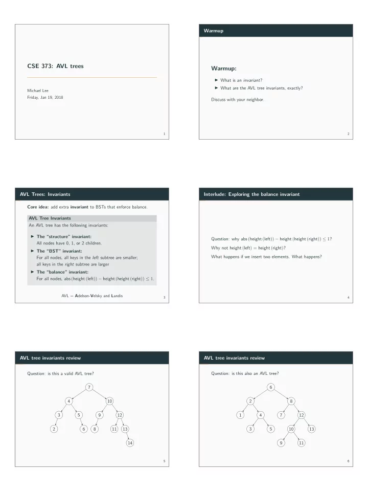
◮ What is an invariant? ◮ What are the AVL tree invariants, exactly? Discuss with your neighbor.
2
AVL Trees: Invariants Core idea: add extra invariant to BSTs that enforce balance. AVL Tree Invariants An AVL tree has the following invariants: ◮ The “structure” invariant: All nodes have 0, 1, or 2 children. ◮ The “BST” invariant: For all nodes, all keys in the left subtree are smaller; all keys in the right subtree are larger ◮ The “balance” invariant: For all nodes, abs (height (left)) − height (height (right)) ≤ 1.
AVL = Adelson-Velsky and Landis
3
Interlude: Exploring the balance invariant Question: why abs (height (left)) − height (height (right)) ≤ 1? Why not height (left) = height (right)? What happens if we insert two elements. What happens?
4
AVL tree invariants review Question: is this a valid AVL tree? 7 4 3 2 5 6 10 9 8 12 11 13 14
5
AVL tree invariants review Question: is this also an AVL tree? 6 2 1 4 3 5 8 7 12 10 9 11 13
6
SLIDE 2 AVL tree invariants review Question: ...and what about now? 8 6 2
5 7 9 11 15
7
Implementing an AVL dictionary How do we implement an AVL dictionary? ◮ get: Same as BST! ◮ containsKey: Same as BST! ◮ put: ??? ◮ remove: ???
8
A basic example Suppose we insert 1, 2, and 3. What happens? insert(1) 1 insert(2) 1 2 insert(3) 1 2 3 What do we do now? Hint: there’s only one possible solution. Rotate. 2 1 3
9
AVL rotation An algorithm for “insert”/“put”, in pictures: Original tree (Balanced) a X b Y Z Insert “c” (Unbalanced!) a X b Y Z c Rotate left (Balanced!) b a X Y Z c
10
Practice Practice: insert 16, and fjx the tree: 15 8 4 3 6 10 22 19 17 20 24
11
Practice Step 1: insert 16 15 8 4 3 6 10 22 19 17 16 20 24
12
SLIDE 3 Practice Step 2: Start from the inserted node and move back up to the
- root. Find the fjrst unbalanced subtree.
15 8 4 3 6 10 22 19 17 16 20 24
13
Practice Step 3: Rotate left or right to fjx. (Here, we rotate right). 15 8 4 3 6 10 19 17 16 22 20 24
14
A second case... Now, try this. Insert 1, 3, then 2. What’s the issue? insert 1 and 3 1 3 insert 2 1 3 2 rotate left 3 1 2 Tree is still unbalanced!
15
The two AVL cases The “line” case The “kink” case
16
Handling the “kink” case Insight: Handling the kink case is hard. Can we somehow convert the kink case into the line case? Solution: Yes, use two rotations!
17
Let’s try again A second attempt... insert 1, 3, 2 (unbalanced!) 1 3 2 double-rotate: convert to line 1 2 3 double-rotate: fix tree 2 1 3
18
SLIDE 4 The kink case: rotation 1 Initial tree (Unbalanced) a W b c Y d X Z Fix the inner “b” subtree: a W c Y d b X Z
19
The kink case: rotation 2 After fjxing the “b” subtree a W c Y d b X Z Fix the outer “a” subtree: c a W Y d b X Z
20
Practice Try inserting a, b, e, c, d into an AVL tree. insert a a insert b a b insert e a b e
21
Practice rotate left on a b a e insert c b a e c insert d b a e c d
22
Practice double rotation on e, part 1 b a e d c double rotation on e, part 2 b a d c e
23
In summary... In summary... Implementing AVL operations ◮ get: Same as BST! ◮ containsKey: Same as BST! ◮ put: Do BST insert, move up tree, perform single or double rotations to balance tree ◮ remove: Either lazy-delete or use similar method to insert
24
SLIDE 5 A note on implementation We sometimes need to rotate left, rotate right, double-rotate left,
Do we need to implement 4 methods? No: can reduce redundancy by having an array of children instead
- f using left or right fjelds. This lets us refer to children by index
so we only have to write two methods: rotate, and double-rotate. (E.g. we can have “rotate” accept two ints: the index to the “bigger” subtree, and the index to the “smaller” subtree)
25
Analyzing Arraylist add
And now, for a completely unrelated topic...
26
Analyzing ArrayList add Exercise: model the worst-case runtime of ArrayList’s add method in terms of n, the number of items inside the list:
public void add(T item) { if (array is full) { resize and copy } this.array[this.size] = item; this.size += 1; }
Answer: T(n) = c when the array is not full n + c when the array is full So, in the WORST possible case, what’s the runtime? Θ (n).
27
Analyzing ArrayList add Question: what’s the runtime on average? Core idea: cost of resizing is amortized over the subsequent calls Metaphors: ◮ When you pay rent, that large cost is amortized over the following month ◮ When you buy an expensive machine, that large cost is amortized and pays itself back over the next several years
28
Analyzing ArrayList’s add Our recurrence: T(n) = c when the array is not full n + c when the array is full Scenario: Let’s suppose the array initially has size k. Let’s also suppose the array initially is at capacity. ◮ How much work do we need to do to resize once then fjll back up to capacity? 1 · (k + c) + (k − 1) · c = k + ck. Note: since array was full, n = k in fjrst resize ◮ What is the average amount of work done? k + ck k = 1 + c
29
Analyzing ArrayList’s add variations Now, what if instead of resizing by doubling, what if we increased the capacity by 100 each time? ◮ Assuming we’re full, how much work do we do in total to resize once then fjll back up to capacity? 1 · (k + c) + 99 · c = k + 100c ◮ What is the average amount of work done? k + 100c 100 = k 100 + c What is k? k is the value of n each time we resize. If we plot this, we’ll get a step-wise function that grows linearly! So, add would be in Θ (n).
30
SLIDE 6 Analyzing ArrayList’s add variations Now, what if instead of resizing by doubling, we triple? ◮ Assuming we’re full, how much work do we do in total to resize once then fjll back up to capacity? 1 · (k + c) + (2k − 1) · c = k + 2kc ◮ What is the average amount of work done? k + 2kc 2k = 1 2 + c So, add would be in Θ (1).
31
Amortized analysis This is called amortized analysis. The technique we discussed: ◮ Aggregate analysis:
Show a series of n operations has an upper-bound of T(n). The average cost is then T(n) n . Other common techniques (not covered in this class): ◮ The accounting method: Assign each operation an “amortized cost”, which may difger from actual cost. If amortized cost > actual cost, incur credit. Credit is later used to pay for operations where amortized cost < actual cost. ◮ The potential method: The data structure has “potential energy”, difgerent operations alter that energy. Hooray, physics metaphors?
32