CSE 101 DISJOINT SET DATA STRUCTURE OPERATIONS WHEN IS WORST-CASE - PowerPoint PPT Presentation
Algorithm Design and Analysis Sanjoy Dasgupta Russell Impagliazzo and Ragesh Jaiswal russell@cs.ucsd.edu Lecture 10: Amortized analysis of Data Structures Thanks, Miles Jones CSE 101 DISJOINT SET DATA STRUCTURE OPERATIONS WHEN IS WORST-CASE
Algorithm Design and Analysis Sanjoy Dasgupta Russell Impagliazzo and Ragesh Jaiswal russell@cs.ucsd.edu Lecture 10: Amortized analysis of Data Structures Thanks, Miles Jones CSE 101
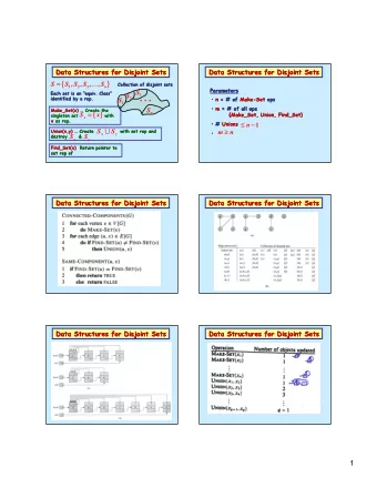
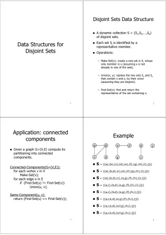
DISJOINT SET DATA STRUCTURE OPERATIONS
WHEN IS WORST-CASE PESSIMISTIC If we are using a data structure operation or other sub-routine, an upper bound for the total time is : !"#$%!&'( ≤ (Number of times operation is performed) (Worst-case time of operation) But this upper bound can be too pessimistic if the time for the operation is highly variable, and ``typical’’ times are much less than worst-case times. (Here, we mean ``typical’’ time through the run of the algorithm even on the worst-case input, not ``for typical inputs’’)
AMORTIZED ANALYSIS Amortized analysis: Bound total time of m operations, rather than worst-case time for single operation * m . Intuition: Fast operations make things worse in the future, but slow operations make things better in the future. (Merging might build up the height of the tree, but finding a deep vertex shrinks the average heights.). Potential function: P_t: Some measure of how bad the situation is after t’th operation. P_0=0, P_t non-negative Today: All potential functions are in terms of ``tokens’’ . We give a token a value v, and charge operations if they hand out tokens, but subtract ``redeemed’’ tokens from amortized time.
AMORTIZED COST OF OPERATION Define ``amortized time’’ of operation j to be !" # = "%&' # + ) # − ) #+, "-./0!&-1.%2'3"%&' = !" , + !" 4 + ⋯ !" 6 = "%&' , − ) 7 + ) , + "%&' 4 − ) , + ) 4 + "%&' 8 − ) 4 + ) 8 + ⋯ . "%&' 6 − ) 6+, + )& = "-./0"%&' + ) 6 − ) 7 ≥ Total time since ) 7 = 0, ) 6 ≥ 0
AMORTIZED TIME BOUNDS TOTAL TIME Thus, the total amortized time is an upper bound on the total time of all operations. Then the total time for m operations is at most m* Worst-case amortized time of an operation In other words, worst-case ``amortized’’ time can be a tighter bound on ``average time’’ for data structure operations. Averaging is over a sequence of operations, not over random inputs.
SIMPLE EXAMPLE: MERGE Say we write the merge algorithm, which combines two sorted lists into one as: Merge[A[1..n], B[1..m]] I= 1 , J =1, K=1 While I ≤ " #"$ % ≤ & $': While B[J] < A[I] do: C[K]=B[J], J++, K++ C[K]=A[I], I++, K++ If I > n, copy rest of B into C, else copy rest of A into C There are two nested loops, inside has worst-case time O(m), outside loops up to n times. However, actual worst-case time is O(m+n)
AMORTIZED ANALYSIS USING TOKENS I= 1 , J =1, K=1. Give tokens worth C= inside while time to each B[J] While I ≤ " #"$ % ≤ & $': While B[J] < A[I] do: C[K]=B[J], J++, K++, remove token from B[J] C[K]=A[I], I++, K++ If I > n, copy rest of B into C, else copy rest of A into C Initialization: Amortized time O(m) Each step in inside while, except last, is paid for with token. Amortized time for inside while = O(1). Total amortized time : O(m) +n O(1) = O(m+n).
SIMPLE EXAMPLE: CASH REGISTER Bills have powers of 10 denominations, 1, 10, 100, 1000, 10000 When we reach 10 of one denomination, trade in for larger. Bills deposited one at a time. If m bills are deposited, and the register starts empty, bound the total number of trades.
WORST-CASE FOR ONE DEPOSIT If we have n consecutive denominations each with 9 bills, one deposit could cause n trades. But that situation needs to be built towards. Let the tokens be the bills in the register, and make them worth v, for a value of v we’ll solve for later.
AMORTIZED TRADES FOR ONE DEPOSIT Each time we trade in bills, we take 9 bills and replace them by 1. Amortized time of that is 1 swap – 8 v since the number of tokens went # down by v. Let’s set ! = $ , &'()*+ ,ℎ). '&/0,)123 4/., 0. Any deposit then has an immediate amortized cost of v=1/8 followed by a series of swaps, which each have amortized cost 0, so all deposits have amortized cost 1/8 # That means, the total number of swaps ≤ $ ,/,'8 *9&:20 /; 32</.),.. No matter what sequence of deposits get made.
DATA STRUCTURES FOR DISJOINT SETS Last time, we came up with a pretty good data structure to keep track of a partition of objects into disjoint sets, which worked well in Kruskal’s algorithm. We showed that Find took at most O(log |V|) time, and Union constant time. But then we had an idea for an improvement, called Path Compression. We asked: how much of a difference could Path Compression take? It doesn’t improve worst-case time for Find, but could it improve amortized time? If so, by how much?
VERSION 2C: DSDS OPERATIONS Find(v). Time = O(depth ) As we find the ancestors of v, we make them point directly to the leader. If p(v) is not v, p(v)=Find(p(v)). Return p(v) . We make smaller ``depth’’ root the child of the other. Union(u, v). Still O(1) time If rank(u) > rank(v) Then: p(v)= u; If rank(u) < rank(v). Then: p(u)=v If rank(u)=rank(v). Then p(v)=u, rank(u)++ Note: rank might no longer= depth, because path compression might flatten tree. Still an upper bound on depth.
DIGRESSION: VERY FAST GROWING AND VERY SLOW GROWING FUNCTIONS We saw how fast the exponential function grew. 2 "## $% &$''() *ℎ,- *ℎ( *$.( %*(/% $- *ℎ( 0-$1()%( 2 % ℎ$%*3)4. The inverse of the exponential function is the log - function. It goes to infinity, but relatively slowly. log *$.( $- 0-$1()%( 2 % ℎ$%*3)4 ≤ 200 Can you think of any functions that are even faster growing than exponential? What does that say about their inverses?
FUNCTIONS FASTER THAN EXPONENTIAL Some functions that are faster growing than 2 " #$%ℎ' () 4 " , , " , ,!, ./ 2 " 0 . I would still call these exponential type functions, but either the base or the exponent is bigger. How about a function that is to exponential as exponential is to polynomial?
DOUBLE EXPONENTIAL How about exponential in an exponential quanity? F(n) = 2 " # . grows amazingly fast. F(200) = 2 " $%% = ' ()*+,- ./) 0/)12( 3 4 5-64, 4ℎ, +6('-. ,89'(:6/( /; 6; ,<,-. 46*, Step in history you wrote down a bit. The inverse function is log(log (). log log number of times in history ≤ log 200 ≤ 8
KEEP GOING TE(n)= 2 " #$ , &'()*+) &+ log(log(log(' ) ) ) FE(n) = 2 " ##$ , inverse is log (log (log (log (n)))) We can keep defining such functions, and each one is exponentially larger than the previous one. Can any function be faster than all of these at once?
SURE The tower function, T(n) is defined by T(1)=2, T(n+1)= 2 " # . In other words, T(n) is a tower of exponentials n high. T(1) =2, T(2) = 4, T(3) =16, T(4) = 256, T(5) is bigger than the universe, T(6) is too long to write in the universe, T(7) is too long to write in every multiverse, assuming quantum physics has split the universe into parallel universes every time step in history, T(8) is exponential in that number,….. The inverse of the tower function is called log ∗ ( . You can compute it as log ∗ ( = 1 +, ( ≤ 2, log ∗ ( = 1 + log ∗ (log () 23ℎ567+85.
CONSTANT FOR PRACTICAL PURPOSES While in principle log ∗ % grows to infinity as n goes to infinity, you are pretty safe assuming say log ∗ % ≤ 6. Could such a function come up in algorithm analysis? Yes, it happens more often than you’d think. We’ll prove a log ∗ ) . Upper bound on the amortized complexity of the union find data structure with path compression.
VARIANTS Let b > 1. We can define a base b version of tower function: ! " 1 = %, ! " ' + 1 = % ) * (,) . While ! " ' can be much smaller than T(n) for b < 2, the height of the tower is more important than the base, so the inverse function ∗ ' ≤ log ∗ ' + 3 . For some constant C. log " ∗ We’ll show an upper bound of log 4 ' but that is the same order as 5 log ∗ '
TOKENS To do a similar analysis for union-find, imagine giving out coupons to the elements. The larger the size field, the more coupons the element will have. Each coupon will be worth ``one free pointer change’’ for a future operation. In other words, if the time for the find operation is C+ C’ (depth of vertex found), we’ll set v= C’. We’ll give rules in terms of the algorithm for handing out and using coupons, but these are just for the analysis; the algorithm itself does not change.
RULES FOR TOKENS Make set: Give the new element 2 tokens Merge: The root that becomes the child gives the one that becomes its parent half of its tokens , round down. If the number at the child was odd, the token protocol gives the parent one more (so the parent gets half the child’s tokens, round up) Find: If a vertex’s pointer changes, and it has at least one token, it spends that token P_t = C * Total tokens on all vertices at time t, where C is time to change a pointer and look-up parent pointer.
VERSION 2C: DSDS OPERATIONS WITH TOKENS Find(v). If p(L) is not L: If L has tokens, and p(L) is not the root, spend one of L’s tokens p(L)=Find(p(L)). Return p(L) . We make smaller depth root the child of the other. Union(u, v). If rank(u) > rank(v) Then: p(v)= u; Move half of v’s tokens to u If rank(u) < rank(v). Then: p(u)=v. Move half of u’s tokens to v If rank(u)=rank(v). Then p(v)=u, rank(u)++ Move 1/2 v’s tokens to u
Recommend
More recommend
Explore More Topics
Stay informed with curated content and fresh updates.
