CS70: Lecture 33. Inequalities: An Overview Chebyshev Distribution - - PowerPoint PPT Presentation

CS70: Lecture 33.

WLLN, Confidence Intervals (CI): Chebyshev vs. CLT

• 1. Review: Inequalities: Markov, Chebyshev
• 2. Law of Large Numbers
• 3. Review: CLT
• 4. Confidence Intervals: Chebyshev vs. CLT

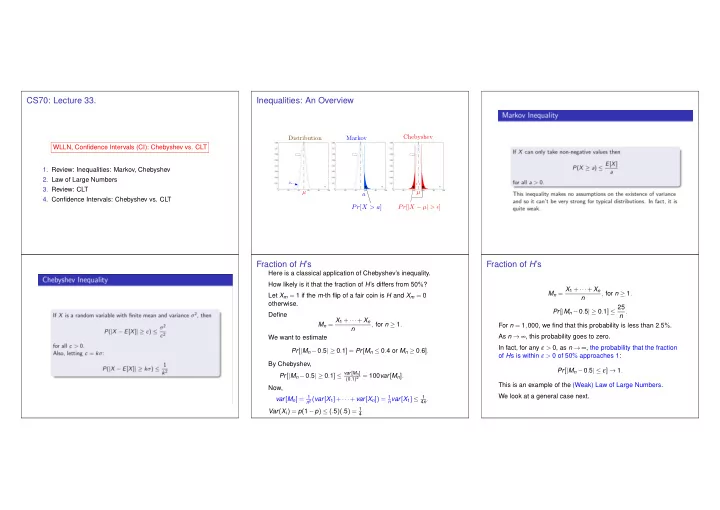
Inequalities: An Overview

n pn

µ Pr[|X − µ| > ]

• Chebyshev

n pn

pn

Distribution

n pn

Pr[X > a] a Markov µ

Fraction of H’s

Here is a classical application of Chebyshev’s inequality. How likely is it that the fraction of H’s differs from 50%? Let Xm = 1 if the m-th flip of a fair coin is H and Xm = 0

• therwise.

Define Mn = X1 +···+Xn n , for n ≥ 1. We want to estimate Pr[|Mn −0.5| ≥ 0.1] = Pr[Mn ≤ 0.4 or Mn ≥ 0.6]. By Chebyshev, Pr[|Mn −0.5| ≥ 0.1] ≤ var[Mn]

(0.1)2 = 100var[Mn].

Now, var[Mn] = 1

n2 (var[X1]+···+var[Xn]) = 1 nvar[X1] ≤ 1 4n.

Var(Xi) = p(1−p) ≤ (.5)(.5) = 1

4

Fraction of H’s

Mn = X1 +···+Xn n , for n ≥ 1. Pr[|Mn −0.5| ≥ 0.1] ≤ 25 n . For n = 1,000, we find that this probability is less than 2.5%. As n → ∞, this probability goes to zero. In fact, for any ε > 0, as n → ∞, the probability that the fraction

• f Hs is within ε > 0 of 50% approaches 1:

Pr[|Mn −0.5| ≤ ε] → 1. This is an example of the (Weak) Law of Large Numbers. We look at a general case next.

Weak Law of Large Numbers

Theorem Weak Law of Large Numbers Let X1,X2,... be pairwise independent with the same distribution and mean µ. Then, for all ε > 0, Pr[|X1 +···+Xn n − µ| ≥ ε] → 0, as n → ∞. Proof: Let Mn = X1+···+Xn

n

. Then Pr[|Mn − µ| ≥ ε] ≤ var[Mn] ε2 = var[X1 +···+Xn] n2ε2 = nvar[X1] n2ε2 = var[X1] nε2 → 0, as n → ∞.

Recap: Normal (Gaussian) Distribution.

For any µ and σ, a normal (aka Gaussian) random variable Y, which we write as Y = N (µ,σ2), has pdf fY(y) = 1 √ 2πσ2 e−(y−µ)2/2σ2. Standard normal has µ = 0 and σ = 1. Note: Pr[|Y − µ| > 1.65σ] = 10%;Pr[|Y − µ| > 2σ] = 5%.

Recap: Central Limit Theorem

Central Limit Theorem Let X1,X2,... be i.i.d. with E[X1] = µ and var(X1) = σ2. Define Sn := An − µ σ/√n = X1 +···+Xn −nµ σ√n . Then, Sn → N (0,1),as n → ∞. That is, Pr[Sn ≤ α] → 1 √ 2π

α

−∞ e−x2/2dx.

E(Sn) = 1 σ/√n(E(An)− µ) = 0 Var(Sn) = 1 σ2/nVar(An) = 1.

Confidence Interval (CI) for Mean: CLT

Let X1,X2,... be i.i.d. with mean µ and variance σ2. Let An = X1 +···+Xn n . The CLT states that An − µ σ/√n = X1 +···+Xn −nµ σ√n → N (0,1) as n → ∞. Thus, for n ≫ 1, one has Pr[−2 ≤ (An − µ σ/√n ) ≤ 2] ≈ 95%. Equivalently, Pr[µ ∈ [An −2 σ √n,An +2 σ √n]] ≈ 95%. That is, [An −2 σ √n,An +2 σ √n] is a 95%−CI for µ.

CI for Mean: CLT vs. Chebyshev

Let X1,X2,... be i.i.d. with mean µ and variance σ2. Let An = X1 +···+Xn n . The CLT states that X1 +···+Xn −nµ σ√n → N (0,1) as n → ∞. Also, [An −2 σ √n,An +2 σ √n] is a 95%−CI for µ. What would Chebyshev’s bound give us? [An −4.5 σ √n,An +4.5 σ √n] is a 95%−CI for µ.(Why?) Thus, the CLT provides a smaller confidence interval.

Coins and CLT.

Let X1,X2,... be i.i.d. B(p). Thus, X1 +···+Xn = B(n,p). Here, µ = p and σ =

• p(1−p). CLT states that

X1 +···+Xn −np

• p(1−p)n

→ N (0,1).

Coins and CLT.

Let X1,X2,... be i.i.d. B(p). Thus, X1 +···+Xn = B(n,p). Here, µ = p and σ =

• p(1−p). CLT states that

X1 +···+Xn −np

• p(1−p)n

→ N (0,1) and [An −2 σ √n,An +2 σ √n] is a 95%−CI for µ with An = (X1 +···+Xn)/n. Hence, [An −2 σ √n,An +2 σ √n] is a 95%−CI for p. Since σ ≤ 0.5, [An −20.5 √n,An +20.5 √n] is a 95%−CI for p. Thus, [An − 1 √n,An + 1 √n] is a 95%−CI for p.

Summary

Inequalities and Confidence Interals

• 1. Inequalities: Markov and Chebyshev Tail Bounds
• 2. Weak Law of Large Numbers
• 3. Confidence Intervals: Chebyshev Bounds vs. CLT Approx.
• 4. CLT: Xn i.i.d. =

⇒ An−µ

σ/√n → N (0,1)

• 5. CI: [An −2 σ

√n,An +2 σ √n] = 95%-CI for µ.