CS156: The Calculus of Given Theories T i over signatures i - PowerPoint PPT Presentation

Combining Decision Procedures: Nelson-Oppen Method CS156: The Calculus of Given Theories T i over signatures Σ i Computation with corresponding decision procedures P i for T i -satisfiability. Zohar Manna Goal Winter 2010 Decide satisfiability of a formula F in theory ∪ i T i . Example : How do we show that F : 1 ≤ x ∧ x ≤ 2 ∧ f ( x ) � = f (1) ∧ f ( x ) � = f (2) is ( T E ∪ T Z )-unsatisfiable? 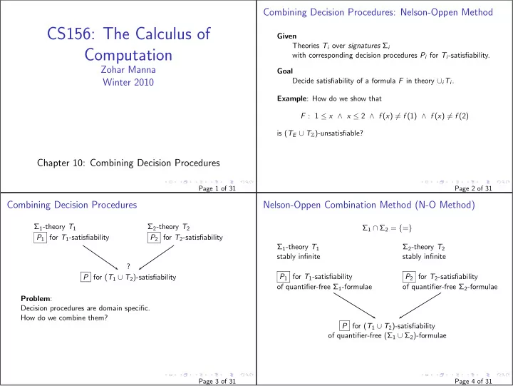Chapter 10: Combining Decision Procedures Page 1 of 31 Page 2 of 31 Combining Decision Procedures Nelson-Oppen Combination Method (N-O Method) Σ 1 -theory T 1 Σ 2 -theory T 2 Σ 1 ∩ Σ 2 = { = } P 1 for T 1 -satisfiability P 2 for T 2 -satisfiability Σ 1 -theory T 1 Σ 2 -theory T 2 stably infinite stably infinite ? P 1 for T 1 -satisfiability P 2 for T 2 -satisfiability P for ( T 1 ∪ T 2 )-satisfiability of quantifier-free Σ 1 -formulae of quantifier-free Σ 2 -formulae Problem : Decision procedures are domain specific. How do we combine them? P for ( T 1 ∪ T 2 )-satisfiability of quantifier-free (Σ 1 ∪ Σ 2 )-formulae Page 3 of 31 Page 4 of 31

Nelson-Oppen: Limitations Stably Infinite Theories Given formula F in theory T 1 ∪ T 2 . A Σ-theory T is stably infinite iff for every quantifier-free Σ-formula F : 1. F must be quantifier-free. if F is T -satisfiable 2. Signatures Σ i of the combined theory only share =, i.e., then there exists some T -interpretation that satisfies F with infinite domain Σ 1 ∩ Σ 2 = { = } 3. Theories must be stably infinite. Example: Σ-theory T Σ : { a , b , = } Note: Axiom ◮ Algorithm can be extended to combine arbitrary number of ∀ x . x = a ∨ x = b theories T i — combine two, then combine with another, and so on. For every T -interpretation I , | D I | ≤ 2 (by the axiom — at most ◮ We restrict F to be conjunctive formula — otherwise convert two elements). Hence, T is not stably infinite. to equivalent DNF and check each disjunct. All the other theories mentioned so far are stably infinite. Page 5 of 31 Page 6 of 31 Example: T E is stably infinite Example Consider quantifier-free conjunctive (Σ E ∪ Σ Z )-formula Proof. Let F be T E -satisfiable quantifier-free Σ E -formula F : 1 ≤ x ∧ x ≤ 2 ∧ f ( x ) � = f (1) ∧ f ( x ) � = f (2) . with arbitrary satisfying T E -interpretation I : ( D I , α I ). α I maps = to = I . The signatures of T E and T Z only share =. Also, both theories are Let A be any infinite set disjoint from D I . Construct new stably infinite. Hence, the N-O combination of the decision interpretation J : ( D J , α J ) such that procedures for T E and T Z decides the ( T E ∪ T Z )-satisfiability of F . ◮ D J = D I ∪ A Intuitively, F is ( T E ∪ T Z )-unsatisfiable. ◮ α J agrees with α I : the extension of functions and predicates For the first two literals imply x = 1 ∨ x = 2 so that for A is irrelevant, except = J . For v 1 , v 2 ∈ D J , f ( x ) = f (1) ∨ f ( x ) = f (2).  v 1 = I v 2 if v 1 , v 2 ∈ D I Contradict last two literals.   Hence, F is ( T E ∪ T Z )-unsatisfiable.  v 1 = J v 2 ≡ true if v 1 is the same element as v 2   false otherwise  J is a T E -interpretation satisfying F with infinite domain. Hence, T E is stably infinite. Page 7 of 31 Page 8 of 31

Nelson-Oppen Method: Overview Phase 1: Variable abstraction Consider quantifier-free conjunctive (Σ 1 ∪ Σ 2 )-formula F . Given quantifier-free conjunctive (Σ 1 ∪ Σ 2 )-formula F . Transform F into two quantifier-free conjunctive formulae Two versions: ◮ nondeterministic — simple to present, but high complexity Σ 1 -formula F 1 and Σ 2 -formula F 2 ◮ deterministic — efficient s.t. F is ( T 1 ∪ T 2 )-satisfiable iff F 1 ∧ F 2 is ( T 1 ∪ T 2 )-satisfiable Nelson-Oppen (N-O) method proceeds in two steps: ◮ Phase 1 (variable abstraction) F 1 and F 2 are linked via a set of shared variables: — same for both versions shared( F 1 , F 2 ) = free( F 1 ) ∩ free( F 2 ) ◮ Phase 2 nondeterministic: guess equalities/disequalities and check deterministic: generate equalities/disequalities by equality For term t , let hd( t ) be the root symbol, e.g. hd( f ( x )) = f . propagation Page 9 of 31 Page 10 of 31 Generation of F 1 and F 2 Example For i , j ∈ { 1 , 2 } and i � = j , repeat the transformations Consider (Σ E ∪ Σ Z )-formula (1) if function f ∈ Σ i and hd( t ) ∈ Σ j , F : 1 ≤ x ∧ x ≤ 2 ∧ f ( x ) � = f (1) ∧ f ( x ) � = f (2) . F [ f ( t 1 , . . . , t , . . . , t n )] ⇒ F [ f ( t 1 , . . . , w , . . . , t n )] ∧ w = t By transformation 1, since f ∈ Σ E and 1 ∈ Σ Z , (2) if predicate p ∈ Σ i and hd( t ) ∈ Σ j , replace f (1) by f ( w 1 ) and add w 1 = 1. Similarly, replace f (2) by f ( w 2 ) and add w 2 = 2. F [ p ( t 1 , . . . , t , . . . , t n )] ⇒ F [ p ( t 1 , . . . , w , . . . , t n )] ∧ w = t Hence, construct the Σ Z -formula (3) if hd( s ) ∈ Σ i and hd( t ) ∈ Σ j , F Z : 1 ≤ x ∧ x ≤ 2 ∧ w 1 = 1 ∧ w 2 = 2 F [ s = t ] ⇒ F [ w = t ] ∧ w = s and the Σ E -formula F [ s � = t ] ⇒ F [ w � = t ] ∧ w = s F E : f ( x ) � = f ( w 1 ) ∧ f ( x ) � = f ( w 2 ) . where w is a fresh variable in each application of a transformation. F Z and F E share the variables { x , w 1 , w 2 } . F Z ∧ F E is ( T E ∪ T Z )-equisatisfiable to F . Page 11 of 31 Page 12 of 31

Example Nondeterministic Version Consider (Σ E ∪ Σ Z )-formula Phase 2: Guess and Check ◮ Phase 1 separated (Σ 1 ∪ Σ 2 )-formula F into two formulae: F : f ( x ) = x + y ∧ x ≤ y + z ∧ x + z ≤ y ∧ y = 1 ∧ f ( x ) � = f (2) . In the first literal, hd( f ( x )) = f ∈ Σ E and hd( x + y ) = + ∈ Σ Z ; Σ 1 -formula F 1 and Σ 2 -formula F 2 thus, by (3), replace the literal with ◮ F 1 and F 2 are linked by a set of shared variables: w 1 = x + y ∧ w 1 = f ( x ) . In the final literal, f ∈ Σ E but 2 ∈ Σ Z , so by (1), replace it with V = shared( F 1 , F 2 ) = free( F 1 ) ∩ free( F 2 ) f ( x ) � = f ( w 2 ) ∧ w 2 = 2 . ◮ Let E be an equivalence relation over V . Now, separating the literals results in two formulae: ◮ The arrangement α ( V , E ) of V induced by E is: F Z : w 1 = x + y ∧ x ≤ y + z ∧ x + z ≤ y ∧ y = 1 ∧ w 2 = 2 � α ( V , E ) : u = v is a Σ Z -formula, and u , v ∈ V . uEv F E : w 1 = f ( x ) ∧ f ( x ) � = f ( w 2 ) � ∧ u � = v is a Σ E -formula. u , v ∈ V . ¬ ( uEv ) The conjunction F Z ∧ F E is ( T E ∪ T Z )-equisatisfiable to F . Page 13 of 31 Page 14 of 31 Nondeterministic Version Example 1 Lemma Consider (Σ E ∪ Σ Z )-formula the original formula F is ( T 1 ∪ T 2 )-satisfiable iff there exists an equivalence relation E over V s.t. F : 1 ≤ x ∧ x ≤ 2 ∧ f ( x ) � = f (1) ∧ f ( x ) � = f (2) (1) F 1 ∧ α ( V , E ) is T 1 -satisfiable, and Phase 1 separates this formula into the Σ Z -formula (2) F 2 ∧ α ( V , E ) is T 2 -satisfiable. Otherwise, F is ( T 1 ∪ T 2 )-unsatisfiable. F Z : 1 ≤ x ∧ x ≤ 2 ∧ w 1 = 1 ∧ w 2 = 2 and the Σ E -formula F E : f ( x ) � = f ( w 1 ) ∧ f ( x ) � = f ( w 2 ) with V = shared( F 1 , F 2 ) = { x , w 1 , w 2 } There are 5 equivalence relations over V to consider, which we list by stating the partitions: Page 15 of 31 Page 16 of 31

Example 1 Example 2 1. {{ x , w 1 , w 2 }} , i.e. , x = w 1 = w 2 : Consider the (Σ cons ∪ Σ Z )-formula x = w 1 and f ( x ) � = f ( w 1 ) ⇒ F E ∧ α ( V , E ) is T E -unsatisfiable. F : car( x ) + car( y ) = z ∧ cons( x , z ) � = cons( y , z ) . 2. {{ x , w 1 } , { w 2 }} , i.e. , x = w 1 , x � = w 2 : x = w 1 and f ( x ) � = f ( w 1 ) ⇒ F E ∧ α ( V , E ) is T E -unsatisfiable. After two applications of (1), Phase 1 separates F into the 3. {{ x , w 2 } , { w 1 }} , i.e. , x = w 2 , x � = w 1 : Σ cons -formula x = w 2 and f ( x ) � = f ( w 2 ) ⇒ F E ∧ α ( V , E ) is T E -unsatisfiable. 4. {{ x } , { w 1 , w 2 }} , i.e. , x � = w 1 , w 1 = w 2 : F c ons : w 1 = car( x ) ∧ w 2 = car( y ) ∧ cons( x , z ) � = cons( y , z ) w 1 = w 2 and w 1 = 1 ∧ w 2 = 2 and the Σ Z -formula ⇒ F Z ∧ α ( V , E ) is T Z -unsatisfiable. 5. {{ x } , { w 1 } , { w 2 }} , i.e. , x � = w 1 , x � = w 2 , w 1 � = w 2 : F Z : w 1 + w 2 = z , x � = w 1 ∧ x � = w 2 and x = w 1 = 1 ∨ x = w 2 = 2 (since 1 ≤ x ≤ 2 implies that x = 1 ∨ x = 2 in T Z ) with ⇒ F Z ∧ α ( V , E ) is T Z -unsatisfiable. V = shared( F cons , F Z ) = { z , w 1 , w 2 } . Hence, F is ( T E ∪ T Z )-unsatisfiable. Page 17 of 31 Page 18 of 31 Example 2 Practical Efficiency Consider the equivalence relation E given by the partition Phase 2 was formulated as “guess and check”: 1. First, guess an equivalence relation E , {{ z } , { w 1 } , { w 2 }} . 2. then check the induced arrangement. The arrangement The number of equivalence relations grows super-exponentially with the # of shared variables. It is given by Bell numbers. α ( V , E ) : z � = w 1 ∧ z � = w 2 ∧ w 1 � = w 2 E.g., 12 shared variables ⇒ over four million equivalence relations. satisfies both F c ons and F Z : Solution: Deterministic Version F c ons ∧ α ( V , E ) is T cons -satisfiable, and F Z ∧ α ( V , E ) is T Z -satisfiable. Hence, F is ( T cons ∪ T Z )-satisfiable. Page 19 of 31 Page 20 of 31