CS156: The Calculus of F [ x 1 , . . . , x n ] or x 1 , . . . , x n - PowerPoint PPT Presentation

Decision Procedures for Quantifier-free Fragments For theory T with signature Σ and axioms A , decide if CS156: The Calculus of F [ x 1 , . . . , x n ] or ∃ x 1 , . . . , x n . F [ x 1 , . . . , x n ] is T -satisfiable Computation � � Decide if Zohar Manna F [ x 1 , . . . , x n ] or ∀ x 1 , . . . , x n . F [ x 1 , . . . , x n ] is T -valid Winter 2008 where F is quantifier-free and free( F ) = { x 1 , . . . 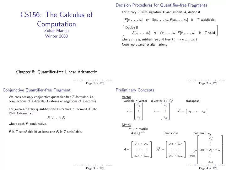, x n } Note: no quantifier alternations Chapter 8: Quantifier-free Linear Arithmetic Page 1 of 125 Page 2 of 125 Conjunctive Quantifier-free Fragment Preliminary Concepts We consider only conjunctive quantifier-free Σ-formulae, i.e., Vector n -vector a ∈ Q n conjunctions of Σ-literals (Σ-atoms or negations of Σ-atoms). variable n -vector transpose     x 1 a 1 For given arbitrary quantifier-free Σ-formula F , convert it into  .   .  a T = � � x = . a = . · · ·     a 1 a n . . DNF Σ-formula     x n a n F 1 ∨ . . . ∨ F k where each F i conjunctive. Matrix m × n -matrix F is T -satisfiable iff at least one F i is T -satisfiable. A ∈ Q m × n transpose column   a 1 j .       . a 11 · · · a 1 n a 11 · · · a m 1  .     . ... . .   . ... . .    A T = . . . . A = a i 1 · · · a ij · · · a in  .   .           .  a m 1 · · · a mn a 1 n · · · a mn row .   .   a mj Page 3 of 125 Page 4 of 125

Multiplication I Multiplication II matrix-matrix vector-vector       . . .   . . . b 1 . . . n        .  � a T b = [ a 1 · · · a n ] .        = a i b i · · · a ik · · · · · · b kj · · ·  = · · · p ij · · ·  .              . . . i =1 . . . b n . . . A B P matrix-vector      � n  where a 11 · · · a 1 n x 1 i =1 a 1 i x i    . .   .   .  ... . . . . b 1 j Ax =  =  . .   .   .  n      . � � �   � n . p ij = a i b j = a i 1 · · · a in  = a ik b kj a m 1 · · · a mn x n i =1 a mi x i  .   k =1 b nj Page 5 of 125 Page 6 of 125 Special Vectors and Matrices Vector Space - set S of vectors closed under addition and scaling of vectors. That is, 0 - vector (column) of 0s if v 1 , . . . , v k ∈ S then λ 1 v 1 + · · · + λ k v k ∈ S 1 - vector of 1s for λ 1 , . . . , λ n ∈ Q n � Thus 1 T x = x i Linear Equation i =1   F : Ax = b 1 0  ...  I =  identity matrix ( n × n )    m × n -matrix variable n -vector m -vector 0 1 represents the Σ Q -formula Thus IA = AI = A , for n × n matrix A . F : ( a 11 x 1 + · · · + a 1 n x n = b 1 ) ∧ · · · ∧ ( a m 1 x 1 + · · · + a mn x n = b m )   0  .  .  .  Gaussian Elimination     Find x s.t. Ax = b by elementary row operations unit vector e i =  1  i th (Note: matrix indices start at 1)   ◮ Swap two rows .   .  .  ◮ Multiply a row by a nonzero scalar   ◮ Add one row to another 0 Page 7 of 125 Page 8 of 125

Example 4 I Example 4 II 1. Add − 2 a 1 + 4 a 2 to a 3 Solve       3 1 2 x 1 6   3 1 2 6       1 0 1 x 2  = 1       1 0 1 1    2 2 1 x 3 2 0 0 1 − 6 Construct the augmented matrix 2. Add − a 1 + 2 a 2 to a 2   3 1 2 6   3 1 2 6   1 0 1 1    0 − 1 1 − 3  2 2 1 2   0 0 1 − 6 Apply the row operations as follows: This augmented matrix is in triangular form. Page 9 of 125 Page 10 of 125 Example 4 III Inverse Matrix Solving A − 1 is the inverse matrix of square matrix A if AA − 1 = A − 1 A = I x 3 = − 6 Square matrix A is nonsingular (invertible) if its inverse A − 1 exists. − x 2 + x 3 = − 3 ⇒ x 2 = − 3 3 x 1 + x 2 + 2 x 3 = 6 ⇒ x 1 = 7 How to compute A − 1 of A ? � � T [ I | A − 1 ] The solution is x = 7 − 3 − 6 [ A | I ] elementary row operations How to compute k th column of A − 1 ? Solve Ay = e k , i.e.  0  . . solve triangular matrix   .     A 1 y = . . .    .  solve using . ( k th column of A − 1 )  .  elementary 0 row operations Page 11 of 125 Page 12 of 125

Linear Inequalities I Linear Inequalities II Convex Space Polyhedral Space An n -dimensional space S ⊆ R n is convex if for all pairs of points For m × n -matrix A , variable n -vector x , and m -vector ¯ b , the v 1 , ¯ ¯ v 2 ∈ S , Σ Q -formula λ ¯ v 1 + (1 − λ )¯ v 2 ∈ S for λ ∈ [0 , 1] . m � G : Ax ≤ ¯ b , i.e. , G : a i 1 x 1 + · · · + a in x n ≤ b i Ax ≤ ¯ v 1 ≤ ¯ b defines a convex space . For suppose A ¯ b and i =1 v 2 ≤ ¯ A ¯ b ; then also describes a subset (space) of Q n , called a polyhedron . v 2 ) ≤ ¯ A ( λ ¯ v 1 + (1 − λ )¯ b . Page 13 of 125 Page 14 of 125 Linear Inequalities III Example I Vertex Consider the linear inequality Consider m × n -matrix A where m ≥ n .     − 1 0 0 0 0 v is a vertex of Ax ≤ ¯ An n -vector ¯ b if there is     0 − 1 0 0 0       x ◮ a nonsingular n × n -submatrix A 0 of A and     0 0 − 1 0 0        y    ◮ corresponding n -subvector ¯ b 0 of ¯ b       0 0 0 − 1 ≤ 0       z 1       such that 1 1 0 0 3         v = ¯ z 2 A 0 ¯ b 0 .     1 0 − 1 0 2   � �� �   The rows a 0 i in A 0 and corresponding values b 0 i of ¯ x b 0 are the set 0 1 0 − 1 2 of defining constraints of the vertex ¯ v . � �� � � �� � A b Two vertices are adjacent if they have defining constraint sets A is a 7 × 4-matrix, b is a 7-vector, and that differ in only one constraint. x is a variable 4-vector representing the four variables { x , y , z 1 , z 2 } . Page 15 of 125 Page 16 of 125

Example II Example III v = [2 1 0 0] T is a vertex of the constraints. For the nonsingular � � T , since Another vertex: v 0 = 0 0 0 0 submatrix A 0 (rows 3, 4, 5, 6 of A : defining constraints of v ),       − 1 0 0 0 0 0       0 0 − 1 0 2 0  0 − 1 0 0   0   0        =  0 0 0 − 1   1   0              0 0 − 1 0 0 0 =             1 1 0 0 0 3       0 0 0 − 1 0 0 1 0 − 1 0 0 2 � �� � � �� � � �� � A 0 v 0 b 0 � �� � � �� � � �� � A 0 v b 0 (rows 1,2,3,4 of A: defining constraints of v 0 ) Note: v and v 0 are not adjacent; they are different in 2 defining constraints. Page 17 of 125 Page 18 of 125 Linear Programming I Linear Programming II Solution: Optimization Problem Find vertex v ∗ satisfying Ax ≤ b and maximizing c T x . max c T x . . . objective function That is, Av ∗ ≤ b and subject to c T v ∗ is maximal: c T v ∗ ≥ c T u for all u satisfying Au ≤ b Ax ≤ b . . . constraints ◮ If Ax ≤ b is unsatisfiable, n then maximum is −∞ � Maximize c i x i ◮ It’s possible that the maximum is unbounded, i =1       then maximum is ∞ a 11 · · · a 1 n x 1 b 1  . ... .   .   .  . . .  ≤ . subject to       . . . .      a m 1 · · · a mn x n b m Page 19 of 125 Page 20 of 125