
SLIDE 1
Cross-diffusion systems with entropy structure
Ansgar J¨ ungel Vienna University of Technology, Austria asc.tuwien.ac.at/∼juengel
1
Introduction and examples
2
Analysis
3
Boundedness-by-entropy method
4
A nonstandard example
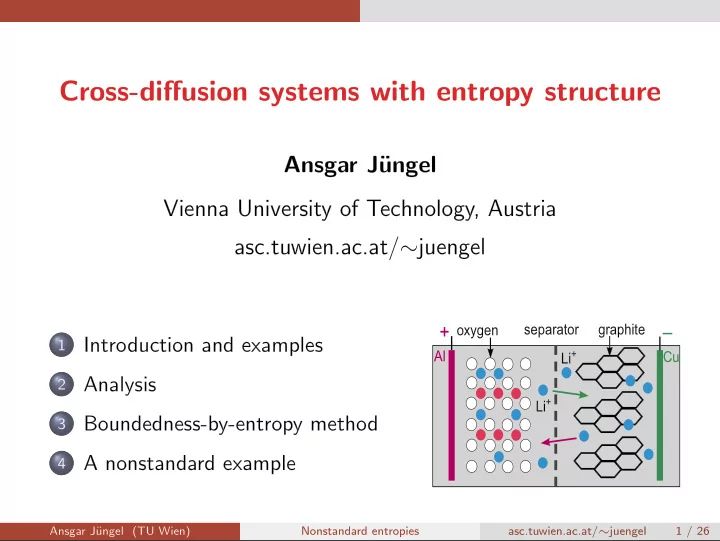
+ –
- xygen
graphite Li+ Li+ Al Cu separator
Ansgar J¨ ungel (TU Wien) Nonstandard entropies asc.tuwien.ac.at/∼juengel 1 / 26