Copulas A copula is the joint distribution of random variables U 1 , - - PowerPoint PPT Presentation

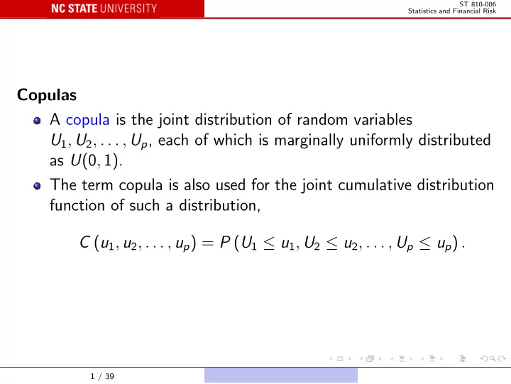
ST 810-006 Statistics and Financial Risk

Copulas A copula is the joint distribution of random variables U1, U2, . . . , Up, each of which is marginally uniformly distributed as U(0, 1). The term copula is also used for the joint cumulative distribution function of such a distribution, C (u1, u2, . . . , up) = P (U1 ≤ u1, U2 ≤ u2, . . . , Up ≤ up) .

1 / 39

ST 810-006 Statistics and Financial Risk

Examples If U1, U2, . . . , Up are independent, C (u1, u2, . . . , up) = u1 × u2 × · · · × up. If they are completely dependent (U1 = U2 = · · · = Up with probability 1), C (u1, u2, . . . , up) = min (u1, u2, . . . , up)

2 / 39

ST 810-006 Statistics and Financial Risk

Sklar’s Theorem Copulas are important because of Sklar’s Theorem:

For any random variables X1, X2, . . . , Xp with joint c.d.f. F(x1, x2, . . . , xp) = P (X1 ≤ x1, X2 ≤ x2, . . . , Xp ≤ xp) and marginal c.d.f.s Fj(x) = P (Xj ≤ x) , j = 1, 2, . . . , p, there exists a copula such that F (x1, x2, . . . , xp) = C [F1 (x1) , F2 (x2) , . . . , Fp (xp)] . If each Fj(x) is continuous, C is unique.

3 / 39

ST 810-006 Statistics and Financial Risk

That is, we can describe the joint distribution of X1, X2, . . . , Xp by the marginal distributions Fj(x) and the copula C. The copula (Latin: link) links the marginal distributions together to form the joint distribution. From a modeling perspective, Sklar’s Theorem allows us to separate the modeling of the marginal distributions Fj(x) from the dependence structure, which is expressed in C.

4 / 39

ST 810-006 Statistics and Financial Risk

The proof is simple in the case that all Fj(x) are continuous, because in this case each has an inverse function F −1

j

(·) such that Fj

• F −1

j

(u)

• = u,

for all 0 ≤ u ≤ 1. If Uj = Fj (Xj), then Uj ∼ U(0, 1): P (Uj ≤ u) = P [Fj (Xj) ≤ u] = P

• Xj ≤ F −1

j

(u)

• = Fj
• F −1

j

(u)

• = u.

Write C for the c.d.f. of this copula; then F (x1, x2, . . . , xp) = P (X1 ≤ x1, X2 ≤ x2, . . . , Xp ≤ xp) = P [U1 ≤ F1 (x1) , U2 ≤ F2 (x2) , . . . , Up ≤ Fp (xp)] = C [F1 (x1) , F2 (x2) , . . . , Fp (xp)] .

5 / 39

ST 810-006 Statistics and Financial Risk

Copula Density When F(·) and C(·) are differentiable, the equation F (x1, x2, . . . , xp) = C [F1 (x1) , F2 (x2) , . . . , Fp (xp)] for the joint cumulative distribution function implies that the joint probability density function (pdf) satisfies f (x1, x2, . . . , xp) f1 (x1) f2 (x2) . . . fp (xp) = c [F1 (x1) , F2 (x2) , . . . , Fp (xp)] where c(·) is the pdf of the copula distribution: c (u1, u2, . . . , up) = ∂p ∂u1∂u2 . . . ∂up C (u1, u2, . . . , up) .

6 / 39

ST 810-006 Statistics and Financial Risk

That is, the copula pdf is the ratio of the joint pdf to what it would have been under independence. So we can also interpret the copula as the adjustment that we need to make to convert the independence pdf into the joint pdf.

7 / 39

ST 810-006 Statistics and Financial Risk

Classes of Copulas An Archimedean copula has the form C(u1, u2, . . . , up) = ψ

• ψ−1(u1) + ψ−1(u2) + · · · + ψ−1(up)
• for an appropriate generator ψ(·).

The Clayton, Frank, Gumbel, and Joe copulas are Archimedean. Each has a single parameter that controls the degree of dependence.

8 / 39

ST 810-006 Statistics and Financial Risk

A copula can be extracted from any joint distribution F(·): C(u1, u2, . . . , up) = F

• F −1

1 (u1), F −1 2 (u2), . . . F −1 p (up)

• Unlike the Pearson (or linear) correlation, the copula is invariant

under monotone increasing transformations of the random variables.

If F(·) is a multivariate normal distribution Np(µ, Σ), then C(·) is a Gaussian copula. If the location or scale of the distribution is changed, the copula does not change, so conventionally µ = 0 and Σ = R, a correlation matrix.

9 / 39

ST 810-006 Statistics and Financial Risk

Gaussian copula for p = 2, ρ = 0.5

0.5 0.5 1 1 1.5 1.5 2 2 2.5 2.5 3 4

0.0 0.2 0.4 0.6 0.8 1.0 0.0 0.2 0.4 0.6 0.8 1.0

Gaussian copula density, rho = 0.5

10 / 39

ST 810-006 Statistics and Financial Risk

Gaussian copula for p = 2, ρ = 0.5

u u cop

Gaussian copula density, rho = 0.5

11 / 39

ST 810-006 Statistics and Financial Risk

If F(·) is a multivariate t-distribution tν(µ, Σ), then C(·) is a t-copula. Again, conventionally µ = 0 and Σ = R, a correlation matrix. But note that when X ∼ tν(µ, Σ):

if ν > 1 then E(X) = µ; if ν > 2 then Var(X) =

• ν

ν − 2

• Σ.

Y =

• ν−2

ν X has the standardized multivariate t-distribution.

12 / 39

ST 810-006 Statistics and Financial Risk

t-copula for p = 2, ν = 5, ρ = 0.5

1 1 2 2 3 3 5 5

0.0 0.2 0.4 0.6 0.8 1.0 0.0 0.2 0.4 0.6 0.8 1.0

t copula density, rho = 0.5 df = 5

13 / 39

ST 810-006 Statistics and Financial Risk

t-copula for p = 2, ν = 5, ρ = 0.5

u u cop

t copula density, rho = 0.5 df = 5

14 / 39

ST 810-006 Statistics and Financial Risk

When R = I, the multivariate normal distribution is that of independent standard normal variables, and the copula has a constant density. But the t-copula still shows dependence.

15 / 39

ST 810-006 Statistics and Financial Risk

t-copula for p = 2, ν = 5, ρ = 0

0.8 0.8 0.8 0.8 1 1 1 1 1.2 1.2 1 . 2 1.2

0.0 0.2 0.4 0.6 0.8 1.0 0.0 0.2 0.4 0.6 0.8 1.0

t copula density, rho = 0 df = 5

16 / 39

ST 810-006 Statistics and Financial Risk

t-copula for p = 2, ν = 5, ρ = 0

u u cop

t copula density, rho = 0 df = 5

17 / 39

ST 810-006 Statistics and Financial Risk

Application to Portfolio Risk Consider a portfolio of p corporate bonds. Ignore interest rate risk, and write the value of bond i at time t when its rating is ρ as Bi(t, ρ). If the rating of bond i at time t is ρi(t), the portfolio value is V (t) =

• i

Bi [t, ρi(t)] . The distribution of the change in value from t to t + δt can be calculated from the joint conditional distribution of ρ1(t + δt), ρ2(t + δt), . . . , ρp(t + δt).

18 / 39

ST 810-006 Statistics and Financial Risk

Historical data give plausible values for the marginal transition probabilities Pρ,ρ′ = P [ρi(t + δt) = ρ′|ρi(t) = ρ] . We can write ρi(t + δt) as a function of a uniform variable Ui: ρi(t + δt) = ρ′, where ρ′ satisfies P [ρi(t + δt) < ρ′|ρi(t)] < Ui ≤ P [ρi(t + δt) ≤ ρ′|ρi(t)] . That is, we break the interval (0, 1) into subintervals with endpoints at the cumulative probabilities P [ρi(t + δt) ≤ ρ′|ρi(t)], and find the subinterval containing Ui.

19 / 39

ST 810-006 Statistics and Financial Risk

To model the joint transition probabilities, we need a joint distribution for U1, U2, . . . , Up. Independence is not plausible: if the bonds were all at the same initial rating, independence implies a multinomial distribution for the counts in the various ratings at a later time, and historical data show considerable over-dispersion relative to the multinomial. We therefore need a copula; the question is, which one?

20 / 39

ST 810-006 Statistics and Financial Risk

The Gaussian Copula Modeling and simulation of dependent transitions is usually described in terms of Gaussian random variables instead of uniform random variables. Write Zi = Φ−1 (Ui), so Zi ∼ N(0, 1), and break the whole real line (−∞, ∞) into subintervals at the Gaussian quantiles corresponding to the cumulative probabilities, Φ−1 {P [ρi(t + δt) ≤ ρ′|ρi(t)]}. Then Zi falls into one of the new subintervals iff Ui falls into the corresponding subinterval of (0, 1), and we can determine the new rating as a function of Zi by finding the subinterval containing Zi.

21 / 39

ST 810-006 Statistics and Financial Risk

The question of what copula to use now becomes: how to model the joint distribution of Z1, Z2, . . . , Zp, given that each of them is marginally N(0, 1). The obvious choice is the multivariate normal distribution Np(0, R) with zero mean vector and with dispersion matrix equal to some correlation matrix R. This is equivalent to using the Gaussian copula defined by Ui = Φ (Zi) , i = 1, 2, . . . , p, where the Z’s have this multivariate normal distribution.

22 / 39

ST 810-006 Statistics and Financial Risk

Choice of R The Gaussian copula for p = 2 has only the single parameter ρ. When p > 2, the 1

2p(p − 1) off-diagonal correlations must be

specified, constrained by the non-negative definiteness of R. When the variables correspond to entities with appropriate structure, a factor model may be used, such as in the Moody’s capital model: Zi = λ1ζG + λ2ζRi + λ3ζIi + λ4ζF,i where λ2

1 + λ2 2 + λ2 3 + λ2 4 = 1, and the ζs are independent

standard normal variables. So each Zi is N(0, 1), and the correlation of Zi and Zj depends

• n which ζs they share.

23 / 39

ST 810-006 Statistics and Financial Risk

Specifically, for i = j, Corr(Zi, Zj) = λ2

1 + λ2 21{Ri=Rj} + λ2 31{Ii=Ij},

where the first term (“global”) is present for all i and j, and the second and third are present for entities in the same region R or industry I, respectively. The resulting correlation matrix R is necessarily non-negative definite.

24 / 39

ST 810-006 Statistics and Financial Risk

In the absence of such structure, general parametric models may be used. An exchangeable correlation matrix has Corr(Zi, Zj) = ρ, i = j. The resulting correlation matrix R is non-negative definite for −1/p ≤ ρ ≤ 1. For ρ ≥ 0, it is the same as the Moody’s model with λ2 = λ3 = 0. An exchangeable correlation matrix may be a reasonable choice when the dependence of all pairs is expected to be the same.

25 / 39

ST 810-006 Statistics and Financial Risk

Sometimes the variables have a natural ordering, such as by time, and nearby variables are expected to be more dependent than widely separated variables. The simplest correlation structure of this form is that of the first

• rder autoregressive model, AR(1):

Corr(Zi, Zj) = φ|i−j| for some φ ∈ [−1, 1]. Like the exchangeable correlation matrix, the AR(1) correlation matrix is characterized by a single parameter, φ.

26 / 39

ST 810-006 Statistics and Financial Risk

Tail Dependence In risk management we are concerned about the tail of the distribution of losses, and often large losses in a portfolio are caused by simultaneous large moves in several components, so

• ne interesting aspect of any copula is the probability it gives to

simultaneous extremes in several dimensions. The lower tail dependence of Xi and Xj is defined as λl = lim

u→0 P

• Xi ≤ F −1

i

(u)|Xj ≤ F −1

j

(u)

• .

It depends only on the copula, and equals lim

u→0

1 uCi,j(u, u).

27 / 39

ST 810-006 Statistics and Financial Risk

Tail dependence is symmetric: the tail dependence of Xi and Xj is the same as that of Xj and Xi. Upper tail dependence λu is defined similarly. The Gaussian copula has the curious property that its tail dependence is 0, regardless of the correlation matrix. The t-copula is similarly derived from the multivariate t-distribution, and has positive tail dependence even when Xi and Xj are uncorrelated: λl = λu = 2tν+1

• −
• (ν + 1)

1 − ρi,j 1 + ρi,j

• where tν+1(·) is the cumulative distribution function of the

univariate t-distribution with ν + 1 degrees of freedom.

28 / 39

ST 810-006 Statistics and Financial Risk

Table : Tail dependence in t-distributions

ρ

• 0.5

0.5 0.9 1 ν = 2 0.058 0.182 0.391 0.718 1 4 0.012 0.076 0.253 0.630 1 10 0.000 0.007 0.082 0.463 1 ∞ 1

29 / 39

ST 810-006 Statistics and Financial Risk

Tail Correlation In some cases, the quantity of interest is the correlation of extreme tail events. Write Ii = 1{Xi≤F −1

i

(u)}.

For instance, Ii could be the indicator of default for the ith bond in a portfolio. Then E(IiIj) = P(Ii = 1 ∩ Ij = 1) = P

• Xi ≤ F −1

i

(u) ∩ Xj ≤ F −1

j

(u)

• = Ci,j(u, u).

30 / 39

ST 810-006 Statistics and Financial Risk

Then Corr(Ii, Ij) = Ci,j(u, u) − u2 u(1 − u) . So the lower tail correlation of Xi and Xj, lim

u→0 Corr(Ii, Ij) = lim u→0

1 uCi,j(u, u), is the same as the lower tail dependence. Similarly for the upper tail correlation.

31 / 39

ST 810-006 Statistics and Financial Risk

Application to CDO Pricing In a CDO (Collateralized Debt Obligation), cash flows from a pool of credit-sensitive instruments are allocated to investors in various tranches, in order of seniority. In a cash CDO, the instruments are bonds, and the investors make initial investments to fund the purchase of the bonds.

32 / 39

ST 810-006 Statistics and Financial Risk

In a synthetic CDO, the instruments are CDSs (Credit Default Swaps).

A CDS duplicates the cash flows of a loan + bond purchase, but without money or bonds changing hands. Since no assets are actually purchased, initial investment is not required (unfunded synthetic CDO). However, in most cases, investors in the lower tranches are required to invest their notional amounts in the vehicle, since they are at most risk of making payments under the pool of CDSs (partially funded synthetic CDO).

33 / 39

ST 810-006 Statistics and Financial Risk

In either type of CDO, an investor in a particular tranche faces a stream of cash flows, say Cj at times tj. Those cash flows have maximum value when no name in the pool defaults, but may be reduced if defaults have occurred. Let τi be the time of default of name i. Then Cj depends on which names have defaulted by time tj: Cj = Cj

• 1{τ1≤tj}, 1{τ2≤tj}, . . . , 1{τN≤tj}
• .

34 / 39

ST 810-006 Statistics and Financial Risk

The value of the tranche is therefore E

• j

e−rtjCj

• ,

where the expected value is with respect to the risk-neutral measure, and r is the risk-free interest rate, assumed to be constant. The marginal risk-neutral distribution of τi can be inferred from the bond market, if this name has issued bonds with the relevant maturities. To construct the full joint risk-neutral distribution, we therefore need a copula.

35 / 39

ST 810-006 Statistics and Financial Risk

The market convention is to use the Gaussian copula with the correlation matrix R =        1 ρ ρ . . . ρ ρ 1 ρ . . . ρ ρ ρ 1 . . . ρ . . . . . . . . . ... . . . ρ ρ ρ . . . 1        . This is known as a single-factor copula, since the underlying Z’s can be constructed as Zi = ζG√ρ + ζname

i

• 1 − ρ,

where ζG ∼ N(0, 1) is common to all Z’s, ζname

i

∼ N(0, 1) is specific to name i, and all ζ’s on the right hand side are independent of each other.

36 / 39

ST 810-006 Statistics and Financial Risk

Since the copula involves only a single parameter, ρ, the resulting risk-neutral distribution can be calibrated to the market price of a single tranche. A first-loss tranche is the first to take losses, up to a detachment point, expressed as a percentage of the pool. A correlation calibrated to a first-loss tranche is called a base correlation. The more senior tranches are characterized by lower and upper detachment (or attachment) points. A correlation calibrated to a non-first-loss tranche is called a compound correlation.

37 / 39

ST 810-006 Statistics and Financial Risk

Unfortunately: Base correlations are found to depend on the detachment point: no one correlation gives prices that match the market price for all detachment points. Instead, they almost always increase with the detachment point. Compound correlations may not be unique: for different values

• f ρ, the expected value matches the market price.

Compound correlations may not even exist: for no value −1 < ρ < 1 does the expected value match the market price.

38 / 39

ST 810-006 Statistics and Financial Risk

Current market practice is to view a non-first-loss tranche as the combination of a long position in the first-loss tranche for the upper detachment point with a short position in the first-loss tranche for the lower detachment (or attachment) point. Its value is then the difference of the values for the two first-loss tranches. That is, two different risk-neutral distributions are used to find the value of a single tranche!

39 / 39