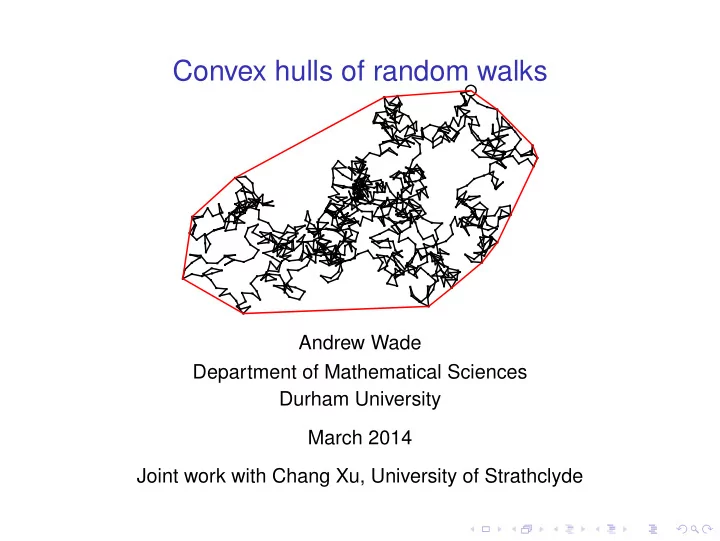
SLIDE 1 Convex hulls of random walks
Department of Mathematical Sciences Durham University March 2014 Joint work with Chang Xu, University of Strathclyde
SLIDE 2 Introduction
On each of n unsteady steps, a drunken gardener drops a
- seed. Once the flowers have bloomed, what is the minimum
length of fencing needed to enclose the garden?
❀ ❀ ❀ ❀ ❀ ❀ ❀ ❀ ❀ ❀ ❀ ❀ ❀ ❀ ❀ ❀ ❀ ❀ ❀ ❀ ❀ ❀ ❀ ❀ ❀ ❀ ❀ ❀ ❀ ❀ ❀ ❀ ❀ ❀ ❀ ❀ ❀ ❀ ❀ ❀ ❀ ❀ ❀ ❀ ❀ ❀ ❀ ❀ ❀ ❀ ❀ ❀ ❀ ❀ ❀ ❀ ❀ ❀ ❀ ❀ ❀ ❀ ❀ ❀ ❀ ❀ ❀ ❀ ❀ ❀ ❀ ❀ ❀ ❀ ❀ ❀ ❀ ❀ ❀ ❀ ❀ ❀ ❀ ❀ ❀ ❀ ❀ ❀ ❀ ❀ ❀ ❀ ❀ ❀ ❀ ❀ ❀ ❀ ❀ ❀
SLIDE 3 Introduction
Let Z1, Z2, . . . be independent, identically distributed random vectors in R2. The Zi will be the increments of the planar random walk Sn, n ≥ 0, defined by S0 = 0 (the origin in R2) and Sn =
n
Zi. We are interested in asymptotic properties of the convex hull hull(S0, . . . , Sn). In particular, the n → ∞ limit behaviour of the random variables Ln = the perimeter length of hull(S0, . . . , Sn).
SLIDE 4 Introduction
Standing assumption: E(Z12) < ∞ (two moments). There is going to be a clear distinction between the zero drift case (EZ1 = 0) and the non-zero drift case (EZ1 > 0). For example, under mild conditions:
- the zero-drift walk is recurrent and the convex hull tends to
the whole of R2;
- the walk with drift is transient with a limiting direction and
the convex hull sits inside some arbitrarily narrow wedge. We will look at both cases in this talk. First, we give a brief summary of some history.
SLIDE 5
1
Introduction
2
Background
3
Zero drift and Brownian scaling limit
4
Non-zero drift and central limit theorem
5
Concluding remarks
SLIDE 6 Some history
Spitzer & Widom (1961) and Baxter (1961) showed that ELn = 2
n
1 k ESk. So, under mild conditions:
- the zero-drift case has ELn ≍ √n;
- the case with drift has ELn ≍ n.
Snyder & Steele (1993) showed that 1 nVar(Ln) ≤ π2 2
. (1) Snyder & Steele deduced from (1) the strong law lim
n→∞ n−1Ln = 2EZ1, a.s.
SLIDE 7 Some questions
The work of Snyder & Steele raised some natural questions.
- Is n the correct order for Var(Ln)?
- Is there a distributional limit theorem for Ln?
- If so, is the limit distribution normal?
The answers to these questions turn out be be essentially
- yes, yes, no in the zero drift case, and
- yes, yes, yes in the non-zero drift case,
excluding some degenerate cases. First, we have a quick look at some simulation evidence.
SLIDE 8 Some simulations
As a concrete example, let Z1 be distributed as (µ, 0) + eΘ, where
- eθ = (cos θ, sin θ) is the unit vector in direction θ;
- Θ is a uniform random variable on [0, 2π).
So EZ1 = (µ, 0), EZ1 = µ. The case µ = 0 is the Pearson–Rayleigh random walk. Picture for µ = 0.2:
SLIDE 9 Some simulations: non-zero drift
- Left: Histogram of Ln samples for n = 104; 106 simulations.
- Right: Plot of point estimates for y = Var(Ln) against
x = n; also shown is the line y = 2x.
200 300 400 500 600 700 10000 20000 30000 40000 50000 60000 70000
150000 250000 0e+00 2e+05 4e+05
Simulations suggest: n−1Var(Ln) → const. (2 in this case!); Ln satisfies a CLT.
SLIDE 10 Some simulations: zero drift
- Left: Histogram of Ln samples for n = 104; 106 simulations.
- Right: Plot of point estimates for y = Var(Ln) against
x = n; also shown is the line y = 0.536x.
100 150 200 250 300 350
- ● ● ● ● ● ● ● ● ●
- ● ● ● ● ● ● ● ●
50000 150000 250000 0e+00 2e+05 4e+05
Simulations suggest: n−1Var(Ln) → const. ≈ 0.536; Ln non-Gaussian limit.
SLIDE 11 First tool: Cauchy formula
Let eθ = (cos θ, sin θ), unit vector in direction θ. Set Mn(θ) = max
0≤k≤n(Sk · eθ),
mn(θ) = min
0≤k≤n(Sk · eθ).
Cauchy’s perimeter formula from convex geometry: Ln = π (Mn(θ) − mn(θ)) dθ.
θ Mn(θ)
SLIDE 12 First tool: Cauchy formula
Ln = π (Mn(θ) − mn(θ)) dθ. A first consequence: classical fluctuation theory for random walk on R gives EMn(θ) =
n
k−1E[(Sk · eθ)+], a formula attributed variously to Kac, Hunt, Dyson, and Chung, and which can be proved combinatorially, or analytically as a consequence of the Spitzer–Baxter fluctuation theory identities. Then ELn =
n
k−1E π |Sk · eθ|dθ = 2
n
k−1ESk, which is the Spitzer–Widom formula.
SLIDE 13 Zero drift case
Suppose EZ1 = 0. The random walk has Brownian motion as its scaling limit. So one would expect that the convex hull of the random walk is described in the limit by the convex hull of Brownian
- motion. The latter was studied
by L´ evy; more recently by El Bachir (1983) and others. We need to know a little about convex hulls of continuous paths, and need to set things up on the right space(s).
SLIDE 14 Paths and hulls
Consider continuous f : [0, T] → Rd with f(0) = 0; say f ∈ C0
d.
(T is not very important—enough to take T ≡ 1.) With the supremum norm ρ∞(f, g) = supx f(x) − g(x) we get a metric space (C0
d, ρ∞).
The path segment (≡ interval image) f[0, t] = {f(s) : s ∈ [0, t]} is compact. = ⇒ hull(f[0, t]) is compact (by a theorem of Carath´ eodory). That is, hull(f[0, t]) is an element of the metric space (K0
d, ρH)
- f compact convex subsets of Rd containing 0, with the
Hausdorff metric.
SLIDE 15
Paths and hulls
Metric space (K0
d, ρH) of compact convex subsets of Rd
containing 0, with the Hausdorff metric. Given A ∈ K0
d and r > 0, let Ar := {x ∈ Rd : ρ(x, A) ≤ r}.
For A, B ∈ K0
d,
ρH(A, B) ≤ r ⇔ A ⊆ Br and B ⊆ Ar.
Lemma 1
For each t, the map f → hull(f[0, t]) is a continuous function from (C0
d, ρ∞) to (K0 d, ρH).
SLIDE 16 Scaling limit
Given random walk Sn = n
i=1 Zi, define
Xn(t) := n−1/2 S⌊nt⌋ + (nt − ⌊nt⌋)
So for each n, Xn ∈ C0
d; Xn(0) = 0 and Xn(1) = n−1/2Sn.
Let bt, t ≥ 0 denote standard Brownian motion on Rd.
Donsker’s Theorem
Suppose E(Z12) < ∞, EZ1 = 0, and E(Z1Z ⊤
1 ) = σ2I, σ2 > 0.
Then Xn/σ ⇒ b in the sense of weak convergence on (C0
d, ρ∞).
Note hull(Xn[0, 1]) = n−1/2 hull(S0, . . . , Sn). Then with Lemma 1 and the continuous mapping theorem, we get:
Theorem 2
Under the same conditions, n−1/2 hull(S0, . . . , Sn) ⇒ hull(b[0, 1]) in the sense of weak convergence on (K0
d, ρH).
SLIDE 17 Functionals
Now take d = 2. One neat way to define perimeter length of a set A ∈ K0
2 is via intrinsic volumes:
L(A) := lim
r↓0
|Ar| − |A| r
where | · | is Lebesgue measure on R2; the limit exists by the Steiner formula of integral geometry. In particular, L(A) =
if int(A) = ∅ 2H1(∂A) if int(A) = ∅ where H1 is one-dimensional Hausdorff measure.
SLIDE 18 Functionals
Lemma 3
The map A → L(A) is a continuous function from (K0
2, ρH) to (R+, ρ).
Note L(Xn[0, 1]) = L(n−1/2 hull(S0, . . . , Sn)) = n−1/2Ln.
Corollary 4
Suppose E(Z12) < ∞, EZ1 = 0, and E(Z1Z ⊤
1 ) = σ2I, σ2 > 0.
Then n−1/2Ln
d
− → ℓ1, where ℓ1 = L(hull(b[0, 1])) is the perimeter length of the convex hull of planar Brownian motion run for unit time. Assuming E(Z12+ε) < ∞, a uniform integrability argument gives lim
n→∞ n−1Var(Ln) = Var(ℓ1).
Work in progress. We can show Var(ℓ1) > 0. We’d like an exact
- formula. Goldman (1996) manages to do a similar calculation for the
planar Brownian bridge, but it is tricky.
SLIDE 19 Non-zero drift case
Now suppose EZ1 > 0. Our results are:
Theorem 5
lim
n→∞
1 nVar(Ln) = 4E[((Z1 − EZ1) · EZ1)2] EZ12 =: s2 ∈ [0, ∞).
Theorem 6
Suppose that s2 > 0. Then for any x ∈ R, lim
n→∞ P
Ln − ELn √VarLn ≤ x
n→∞ P
Ln − ELn √ ns2 ≤ x
the standard normal distribution function.
SLIDE 20
Remarks
(i) A little algebra shows s2 ≤ 4(EZ12 − EZ12). Compare to the Snyder–Steele upper bound n−1Var(Ln) ≤ π2
2 (EZ12 − EZ12).
I.e., the constant in the Snyder–Steele upper bound is not sharp (4 < π2/2). (ii) s2 = 0 if and only if Z1 − EZ1 is a.s. orthogonal to EZ1. This is the case, for instance, if Z1 takes values (1, 1) or (1, −1), each with probability 1/2. In this case Theorem 5 says that Var(Ln) = o(n). The Snyder–Steele bound says only that Var(Ln) ≤ π2n/2. Simulations suggest that actually Var(Ln) = O(log n).
SLIDE 21
Degenerate example
Z1 takes values (1, 1) or (1, −1), each with probability 1/2. This 2-dimensional walk can be viewed as a space-time diagram of a 1-dimensional simple symmetric random walk: Interesting combinatorics here, related to the Bohnenblust–Spitzer algorithm; see Steele (2002). Behaviour of Ln for this case is largely an open problem.
SLIDE 22 Proof idea: Martingale differences
Let Fn = σ(Z1, . . . , Zn). Define Dn,i = E[Ln − L(i)
n | Fi].
Lemma 7
(i) Ln − ELn = n
i=1 Dn,i.
(ii) Var(Ln) = n
i=1 E(D2 n,i).
Sketch proof.
As Z ′
i is independent of Fi, E[L(i) n | Fi] = E[L(i) n | Fi−1] = E[Ln | Fi−1].
So Dn,i = E[Ln | Fi] − E[Ln | Fi−1]; a standard construction of a martingale difference sequence.
n
Dn,i = E[Ln | Fn] − E[Ln | F0] = Ln − ELn. Now use orthogonality of martingale differences.
SLIDE 23 Aside: Upper bounds
Lemma 3 with the conditional Jensen inequality gives: Var(Ln) ≤
n
E[(Ln − L(i)
n )2].
A related result, the Efron–Stein inequality, says Var(Ln) ≤ 1 2
n
E[(Ln − L(i)
n )2].
It is this latter result that Snyder & Steele used to obtain their upper bound.
SLIDE 24 Cauchy formula revisited
We need to study Dn,i = E[Ln − L(i)
n | Fi].
We have the Cauchy formula for Ln, and similarly for L(i)
n , so that
Ln − L(i)
n =
π ∆n,i(θ)dθ, where ∆n,i(θ) =
n (θ)
n (θ)
where, similarly to before, M(i)
n (θ) = max 0≤j≤n(S(i) j
· eθ), m(i)
n (θ) = min 0≤j≤n(S(i) j
· eθ).
SLIDE 25
Proof idea: Control of extrema
We want to understand the relationship between Mn(θ), mn(θ) and M(i)
n (θ), m(i) n (θ) (resampled versions).
WLOG suppose EZ1 = µeπ/2 = (0, µ), where µ > 0. Then for each fixed θ, Sj · eθ is a one-dimensional random walk. Indeed, Sj · eθ = j
k=1 Zk · eθ, with mean increment
E[Z1 · eθ] = E[Z1] · eθ = µ sin θ, which is positive for θ ∈ (0, π). So, with high probability, the maximum Mn(θ) will be achieved nearby step n while the minimum mn(θ) will be achieved nearby step 0. To formalize this needs only the strong law of large numbers, plus some care (need some uniformity in θ).
SLIDE 26 Proof idea: Control of extrema
To get uniform control, take θ ∈ (δ, π − δ). Let Jn(θ) = arg min
0≤j≤n
(Sj · eθ) and Jn(θ) = arg max
0≤j≤n
(Sj · eθ); similarly J(i)
n (θ) and J(i) n (θ) for the walk with Zi resampled.
Let E := En,i(δ, γ) be the event that for all θ ∈ (δ, π − δ),
- Jn(θ) < γn, Jn(θ) > (1 − γ)n;
- J(i)
n (θ) < γn, J(i) n (θ) > (1 − γ)n.
Lemma 8
For any δ ∈ (0, π/2) and γ ∈ (0, 1), P(E) → 1, uniformly in i.
Sketch proof.
Follows from the SLLN.
SLIDE 27
Proof idea: Control of extrema
Lemma 9
On E, ∆n,i(θ) = (Zi − Z ′
i ) · eθ for all i with γn < i < (1 − γ)n.
Sketch proof.
On E, both the J are > (1 − γ)n and both the J are < γn. It follows that for i in the middle, J = J(i) and J = J(i). So mn(θ) = m(i)
n (θ), and
M(i)
n (θ) = S(i) J · eθ = (SJ − Zi + Z ′ i ) · eθ = Mn(θ) + (Z ′ i − Zi) · eθ.
See the picture!
SLIDE 28
Proof idea: Control of extrema
So mn(θ) = m(i)
n (θ), and
M(i)
n (θ) = S(i) J · eθ = (SJ − Zi + Z ′ i ) · eθ = Mn(θ) + (Z ′ i − Zi) · eθ.
See the picture!
SLIDE 29
Finishing the proofs
The main technical work (details omitted!) now is dealing with the error terms (sending δ → 0, γ → 0, n → ∞). Up to these error terms, we have shown that Dn,i = E[Ln − L(i)
n | Fi] ≈
π E[(Zi − Z ′
i ) · eθ | Fi]dθ.
Here Zi is Fi-measurable and Z ′
i is independent of Fi, so
E[(Zi − Z ′
i ) · eθ | Fi] = (Zi − EZ1) · eθ.
Doing the integral gives Dn,i = E[Ln − L(i)
n | Fi] ≈ 2(Zi − EZ1) · EZ1
EZ1 .
SLIDE 30 Finishing the proofs
Formalizing the analysis we get:
Theorem 10
n−1/2
n
2(Zi − EZ1) · EZ1 EZ1
So, perhaps surprisingly, Ln − ELn is well-approximated by a sum of i.i.d. random variables. Theorems 5 and 6 now follow from Theorem 10 easily enough.
SLIDE 31
Concluding remarks
The assumption that the Zi are identically distributed is not essential to the main argument. For example, let Gn =
1 n+1
n
i=0 Si = n i=1 n+1−i n+1 Zi.
G0, G1, . . . is the centre-of-mass process associated with S0, S1, . . .. By convexity, hull(G0, . . . , Gn) ⊆ hull(S0, . . . , Sn). If L⋆
n is the perimeter length of hull(G0, . . . , Gn), then the
statement of Theorem 10 applies to L⋆
n in place of Ln with n+1−i n+1 Zi in place of Zi.
In particular, the analogue of Theorem 5 says that lim
n→∞
1 nVar(L⋆
n) = s2/3,
where s2 is the same as before.
SLIDE 32
Concluding remarks
A picture:
SLIDE 33 Concluding remarks
Ongoing work: look at An, the area of hull(S0, . . . , Sn). There’s a (more complicated) formula for E(An), due to Barndorff-Nielsen and Baxter (1963). We can show
- Var(An) = O(n3) in the case with drift;
- Var(An) = O(n2) in the zero-drift case.
We expect these bounds are of the correct order. There’s a (more complicated) Cauchy formula here, too, but to get a precise limit statement (or even a lower bound) in this case looks harder. Several interesting open problems. . .
SLIDE 34 References
- O. BARNDORFF-NIELSEN & G. BAXTER, Combinatorial lemmas in
higher dimensions, Trans. Amer. Math. Soc. 108 (1963) 313–325.
- G. BAXTER, A combinatorial lemma for complex numbers, Ann. Math.
- Statist. 32 (1961) 901–904.
- M. EL BACHIR, L
’enveloppe convexe du mouvement brownien, Ph.D. thesis, Universit´ e Toulouse III, 1983.
- A. GOLDMAN, Le spectre de certaines mosa¨
ıques poissoniennes du plan et l´ enveloppe convexe du pont brownien, Probab. Theory Relat. Fields 105 (1996) 57–83.
- S.N. MAJUMDAR, A. COMTET, & J. RANDON-FURLING, Random convex
hulls and extreme value statistics, J. Stat. Phys. 138 (2010) 955–1009.
- T.L. SNYDER & J.M. STEELE, Convex hulls of random walks, Proc.
- Amer. Math. Soc. 117 (1993) 1165–1173.
- F. SPITZER & H. WIDOM, The circumference of a convex polygon, Proc.
- Amer. Math. Soc. 12 (1961) 506–509.
- J.M. STEELE, The Bohnenblust–Spitzer algorithm and its applications,
- J. Comput. Appl. Math. 142 (2002) 235–249.
- A.R. WADE & C. XU, Convex hulls of planar random walks with drift,
- Proc. Amer. Math. Soc., arXiv:1301.4059.