Convergence of Ttonnement in Fisher Markets P R E S E N T E D B Y N - PowerPoint PPT Presentation
Convergence of Ttonnement in Fisher Markets P R E S E N T E D B Y N O A A V I G D O R - E L G R A B L I A P R I L 9 , 2 0 1 4 B A S E D O N J O I N T W O R K W I T H Y U V A L R A B A N I Overview Fisher markets
Convergence of Tâtonnement in Fisher Markets P R E S E N T E D B Y N O A A V I G D O R - E L G R A B L I | A P R I L 9 , 2 0 1 4 B A S E D O N J O I N T W O R K W I T H Y U V A L R A B A N I
Overview � ▪ Fisher markets › Definition › Market equilibrium › Eisenberg-Gale convex program ▪ Tâ tonnement ▪ Our results 2
Fisher Markets GOODS AGENTS (Utility func., budget) Prices =? 3
Fisher Markets -- Notation ▪ Consider a marketplace with: • n selfish agents • k perfectly divisible goods ▪ Each agent i =1, 2, … , n has: • Initial budget b i ∈ R + • Utility function u i : X i ⊆ R k + → R + � � Defines the “value” agent i gains � from a basket of goods � ▪ Fisher markets are a special case of the exchange market model of Walras (1874) 4
Market Equilibrium ▪ Given prices p for the goods, the best basket of goods for player i satisfies the following: x i ( p ) = max u i ( x ) Agents maximize s.t : x i · p ≤ e · p b i their utility within the budget constraint x i ∈ X i ▪ Prices p are called market equilibrium iff there exists optimal x i (p) for every agent i such that X X x i ( p ) ≤ 1 e i i i Total demand Total supply 5
Arrow-Debreu Theorem (1954) ▪ In exchange markets with continuous, strictly monotone, and quasi- concave utility functions: a market equilibrium always exists. � ▪ Moreover : every good with positive price is fully consumed � � ▪ In particular this is true for Fisher markets The proof is not constructive 6
Utility Functions ▪ Linear utilities: m Buy only goods with X u ( x ) = a i x i p i /a i minimum . Goods are perfect substitutes i =1 ▪ Leontief utilities: Split the money on all goods (s.t u ( x ) = min i { a i x i } >0) proportional to . p i /a i a i Goods are perfect complements ▪ Cobb-Douglas utilities: k i =1 x a i X u ( x ) = Π k a i = 1 i , s.t i Spend a j b on good j 7
Utility Functions ▪ 𝜍 =1 → linear utilities ∞ ▪ 𝜍 → - → Leontief utilities ▪ 𝜍 → 0 → Cobb-Douglas utilities ▪ CES (Constant Elasticity of substitution) � 1 / ρ 0 1 � @X u ( x ) = ( a j x j ) ρ � A j � Raising the price of one good does not ▪ 0 < 𝜍 ≦ 1 : weak gross substituts decrease the demand for other goods ▪ 𝜍 < 0 : complementary goods Raising the price of one good does not increase the demand for other goods 8
Eisenberg-Gale’s Convex Program [EG ’59, E ’61, KV ’02, CV ’05, JV ‘10] Primal: P n max i =1 b i ln u i ( x i ) P n s.t. i =1 x ij ≤ 1 ∀ j = 1 , 2 , . . . , m x ij ≥ 0 ∀ i = 1 , 2 , . . . , n ; ∀ j = 1 , 2 , . . . , m. The KKT conditions show that Dual: an optimal solution must satisfy the equilibrium conditions P m j =1 p j + P n min i ( µ i ) i =1 g ∗ s.t. i = 1 , 2 , . . . , n ; ∀ j = 1 , 2 , . . . , m p j ≥ − µ ij p j ≥ 0 ∀ j = 1 , 2 , . . . , m, ▪ Eisenberg-Gale markets [JV ’10]: Fisher markets that their equilibrium allocation and prices can be computed using this form of a convex program. 9
Summarize � ▪ Warlas (1874) - Formal definition of a market and a market equilibrium ▪ Arrow-Debreu (1954) - Existence of equilibrium in exchange markets (and in Fisher markets in particular) ▪ Eisenberg-Gale (1959) - Constrictive proof of equilibrium. 10
Tâtonnement [Warlas 1874] This is considered to be a ▪ How do prices converge to equilibrium ? computational process and not a natural market process The tâtonnement process: Prices are lowered for goods with excess supply . Prices are raised for goods with excess demand . The agents always response by demanding an optimal basket at the current prices. � z j ( p ) - the excess demand ▪ The tâtonnement process we consider: of good j with prices p ∀ j = 1 , 2 , . . . , k : p t +1 = p t j (1 + ✏ z j ( p t )) j 11
• convergence Tâtonnement Convergence - Previous Results of the average of the prices. • satisfies only [Arrow, Block, time-continuous process for WGS utilities. the sum of Hurwitz ’59] budget constraint [Scarf ’60] examples of non-WGS utilities for which tâtonnement does not converge. [Codenotti, poly-time convergence of a discrete tâtonnement-like McCune, process for WGS Varadarjan ’05] discrete tâtonnement-like process for a wide range of [Fleisher, Garg, Kapoor, markets but with weak form of convergence. Khandekar ’08] [Cole, Fleisher discrete tâtonnement (similar to ours) for non-linear ‘08] CES utilities that satisfy WGS. [Cheung, Cole, analysis for some non-WGS utilities including Rastogi ’12] complimentary CES utilities with , and multi ρ ∈ ( − 1 , 0) ρ ∈ ( − 1 , 0) level nested CES utilities (with some restrictions). [Cheung, Cole, discrete tâtonnement converge fast for CES utilities Devanaur ’13] with ρ ∈ [ − inf , 0) *WGS - weak gross substitutes 12
Approximate Equilibrium A price-demand pair (p,x) is δ -approximate equilibrium iff : Each agent’s demand • for every agent i : x i = x i ( p ) is optimal given p • For every good j : z j ( p ) < δ The demand for each • For every good j : z j ( p ) < − δ ⇒ p j ≤ δ good doesn’t exceed the supply by much Goods with small demand must have a small price 13
Our Main Theorem β -smooth markets : Prices with dual cost close to optimal have small excess demand for every good ∀ p φ ( p ) ≤ φ ( p ∗ ) + β ( α ) ∀ j | z j ( p ) − z j ( p ∗ ) | ≤ α � ⇒ Which markets are β -smooth � and satisfy conditions C1, C2? � Theorem: For β -smooth markets (given δ >0, for small ε , and large T) φ ( p 0 ) , φ ( p 1 ) , . . . , φ ( p T ) if : C1. is monotonically non-increasing T 0 1 C2. For every T’> T- f( δ , ε ): X z j ( p t ) ≤ β ( δ / 3) 3) ∀ j T 0 + 1 · t =0 then: the pair is δ -approximate equilibrium. ( p T , x T +1 ) 14
Eisenberg-Gale Markets Convergence ▪ Which markets are β smooth and satisfy conditions C1, C2? � Sufficient condition: ɸ (p) is twice continuously differentiable and � strongly convex. � Applying the Theorem : • Given such a market. • Fix a sufficiently small constant ε ✓ − ln p 0 ◆ • For every δ >0, if min T ≥ Ω ✏ 2 � 3 Then is δ -approximate ( p T , x T +1 ) 15
Examples ▪ Using the sufficient condition: ▪ non-linear CES utilities ▪ Exponential utilities: k � X a j (1 − e − θ x j ) u ( x ) = � j =1 � ▪ Using an extended argument: ▪ Leontief ▪ Nested CES-Leontief 16
Interesting Questions ▪ Find tight bounds on the convergence rate ▪ Analyze the convergence of an asynchronous process ▪ Extend this to some Arrow-Debreu markets 17
Thank you! 18
Recommend
More recommend
Explore More Topics
Stay informed with curated content and fresh updates.


