Conventional Surface Water Treatment for Drinking Water Paddle - PowerPoint PPT Presentation

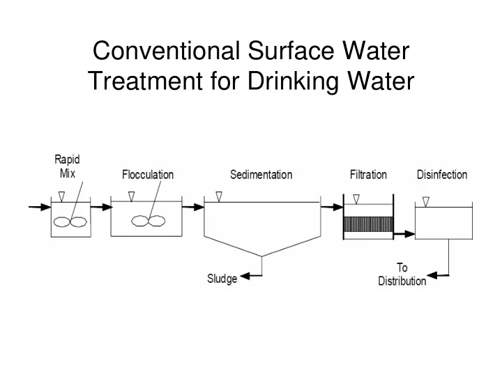
Conventional Surface Water Treatment for Drinking Water

Paddle Flocculators at Everett WTP

The Rate of Collisions by Each Mechanism Can be Predicted from Theory = β r n n floc ij i j π ( ) 2 β = − + DS v v d d ij i j i j 4 ⎛ ⎞ ( ) ( ) 2 k T 1 1 1 3 β = + + ⎜ ⎟ π Br β = + ( )( ) B d d Br g ⎜ ⎟ G d d 3 = ρ − ρ + − µ i j d d d d 3 d d ⎝ ⎠ ij i j µ 6 p w i j i j 72 i j Fluid Shear: Particles on Differential Sedimentation: Brownian Motion: Particles Different Streamlines Travel Particles Collide Due to Collide Due to Random at Different Velocities Different Terminal Velocities Motion

Each mechanism of flocculation is predicted to dominate for certain ranges of particle properties (primarily size)

Considering the short- range interactions leads to a decrease in the predicted flocculation efficiency

Short-range forces are predicted to reduce the effectiveness of shear as a mechanism of flocculation more than the other mechanisms

(From Opflow, June 2000)

( ) d NV ( ) = − + + L ,CV QN Q N dN V r L ,CV p dt Assume pseudo-steady state, so ( ) d NV = L ,CV 0 dt = Q Av 0 = − + 0 Av dN V r 0 L ,CV p = Av dN V r 0 L ,CV p

⎡ ⎤ ⎡ ⎤ Rate of Removal of Particles Number of = − ⎢ ⎥ ⎢ ⎥ V r L ,CV p ⎣ ⎦ ⎣ ⎦ by a Single Collector Collectors in Layer ⎡ ⎤ ⎡ ⎤ ⎡ ⎤ Rate of Approach of Removal Efficiency of Number of = − ⎢ ⎥ ⎢ ⎥ ⎢ ⎥ ⎣ ⎦ ⎣ ⎦ ⎣ ⎦ Particles to a Collector a Single Collector Collectors in Layer ⎡ ⎤ = Nv π 2 Rate of Approach of d c ⎢ ⎥ 0 ⎣ ⎦ Particles to a Collector 4 ⎡ ⎤ ≡ Removal Efficiency of η ⎢ ⎥ ⎣ ⎦ a Single Collector ⎡ ⎤ Total Volume of ⎢ ⎥ ( ) − ε ⎡ ⎤ ⎣ ⎦ Number of AdL 1 Collector Media = = ⎢ ⎥ π ⎡ ⎤ 3 ⎣ ⎦ Volume of a Collectors in Layer d / 6 c ⎢ ⎥ ⎣ ⎦ Single Collector

⎡ ⎤ ⎡ ⎤ ⎡ ⎤ Rate of Approach of Removal Efficiency of Number of = − ⎢ ⎥ ⎢ ⎥ ⎢ ⎥ V r L ,CV p ⎣ ⎦ ⎣ ⎦ ⎣ ⎦ Particles to a Collector a Single Collector Collectors in Layer ( ) ⎡ − ε ⎤ ⎡ ⎤ π 2 AdL 1 d [ ] = − η c ⎢ ⎥ ⎢ ⎥ Nv π 0 3 ⎣ ⎦ ⎣ ⎦ 4 d / 6 c ( ) − ε η “Single Collector 1 3 = − Removal Efficiency” Nv AdL 0 2 d c

= Av dN V r 0 L ,CV p ( ) − ε η 1 3 = − Av dN N v A dL 0 0 2 d c ( ) − ε η 1 dN 3 = − = − λ dL dL N 2 d c “Filter coefficient” N = − λ out ln L N in ( ) = − λ N N exp L out in

Summary: Mass Balance Analysis of Particle Removal in a Granular Filter • Based on relative sizes of particles and collectors, sieving is unimportant and removal can be modeled based on interactions with isolated “collector” grains • Assuming pseudo-steady state, concentration of any given type of particle is expected to decline exponentially with depth • Each type of particle has a different coefficient for the exponential loss rate • If we could predict η for a given type of particle, we could predict N out /N in for that particle

2/3 ⎛ ⎞ k T η = ⎜ ⎟ B 0.905 ⎜ ⎟ µ Br d d v ⎝ ⎠ c p 0

“Filter Ripening”

S=Standard case; L=longer bed; c=concentration; h=headloss

S=Standard case; d=larger diameter grains; c=concentration; h=headloss