Constrained dynamics about anything out of spring systems In - - PowerPoint PPT Presentation

Constrained dynamics

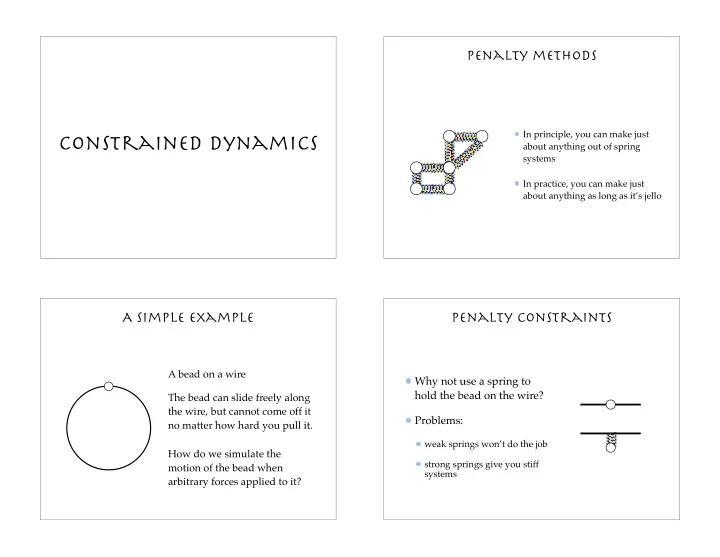
Penalty methods

In principle, you can make just about anything out of spring systems In practice, you can make just about anything as long as it’s jello

A simple example

A bead on a wire The bead can slide freely along the wire, but cannot come off it no matter how hard you pull it. How do we simulate the motion of the bead when arbitrary forces applied to it?

Penalty constraints

Why not use a spring to hold the bead on the wire? Problems:

weak springs won’t do the job strong springs give you stiff systems

fT

First order world

N f fN In this world, f = mv What is the legal velocity? What is the legal force? f = f + ˆ f Add constraint force to cancel the illegal part of f ˆ f ˆ f f

ˆ f = − N · f N · NN

The real world

N In the real world, f = ma What is the legal acceleration? v a depends on both and N v the faster you’re going, the faster you have to turn f ˆ f? Compute such that only generates legal acceleration f ˆ f f = f + ˆ f

Constraint force

All we need is calculate the constraint force In order to calculate constraint force, we need to know what legal acceleration is

Constraints

Implicit: Parametric: θ x C(x) = |x| − r = 0 x = r cos θ sin θ

• r

Legal acceleration

What is the legal position? What is the legal acceleration?

C = 0 ˙ C = 0 ¨ C = 0

˙ C(x) = x · ˙ x = 0 What is the legal velocity? ¨ C(x) = ¨ x · x + ˙ x · ˙ x = 0 C(x) = 1 2x · x − 1 2

Legal conditions

If we start with legal position and velocity We need only ensure the legal acceleration ¨ C(x) = 0 ˙ C(x) = 0 C(x) = 0

C = 0 ˙ C = 0 ¨ C = 0

Constraint force

∂C ∂x · ˆ f = −∂C ∂x · f − m ˙ C ∂x ˙ x

Use the legal condition to compute the constraint force Rewrite the legal condition in a general form

¨ C(x) = ∂ ˙ C ∂x · ˙ x + ∂C ∂x · ¨ x = 0

¨ x = f + ˆ f m

Substitute ¨

x with

¨ C = ∂ ˙ C ∂x · ˙ x + ∂C ∂x · f + ˆ f m

= 0

: constraint gradient ∂C ∂x

Constraint force

∂C ∂x · ˆ f = −∂C ∂x · f − m ˙ C ∂x ˙ x

How many variables do we have? Need one more condition to solve the constraint force

Virtual work

Constraint force is passive - no energy gain or loss

T = 1 2m ˙ x · ˙ x ˙ T = m ˙ x · ¨ x

Kinetic energy of the system:

˙ C(x) = ∂C ∂x · ˙ x = 0

˙ x · ˆ f = 0, ∀ ˙ x | ∂C ∂x · ˙ x = 0

Make sure does no work for every legal velocity: ˆ f Work done by and : f ˆ f

= ˙ x · f + ˙ x · ˆ f

Constraint force

ˆ f = λ∂C ∂x λ = − ∂C

∂x · f − m ∂ ˙ C ∂x · ˙

x

∂C ∂x · ∂C ∂x

˙ x · ˆ f = 0, ∀ ˙ x | ∂C ∂x · ˙ x = 0

must point in the direction of ∂C ∂x ˆ f

∂C ∂x · ˆ f = −∂C ∂x · f − m ˙ C ∂x ˙ x

Substituting for in ˆ f

The Bead Example

N v f ˆ f?

ˆ f = λ∂C ∂x λ = − ∂C

∂x · f − m ∂ ˙ C ∂x · ˙

x

∂C ∂x · ∂C ∂x

Geometric view

f ˆ f

When the system is at rest,

ˆ f = − N · f N · NN N N = ∂C ∂x

Differentiating gives a normal vector C What about the case when is nonzero? ˙ x

λ = − ∂C

∂x · f − m ∂ ˙ C ∂x · ˙

x

∂C ∂x · ∂C ∂x

Geometric view

N ¨ x = f + ˆ f m = f m − f · N mN · NN − ˙ N · ˙ x N · NN a ax ¨ x = ax − ˙ N · ˙ x N · NN λ = − ∂C

∂x · f − m ∂ ˙ C ∂x · ˙

x

∂C ∂x · ∂C ∂x

In principle, ensuring legal acceleration can keep the particle exactly on the circle In practice, two problems cause the particle to drift

numerical errors can accumulate when the ODE is not solved exactly constraints might not be met initially

A feedback term handles both problems:

Feedback

¨ C = −ksC − kd ˙ C instead of ¨ C = 0

Tinkertoys

Now we know how to simulate a bead on a wire Apply the simple idea, we can create a constrained particle system

Constrained particle systems

Particles: points in phase space Multiple constraints

Each is a function Ci(x1, x2, . . .) Constraint force: linear combination of constraint gradients ∂Ci

∂x , ∀i

Legal state: Ci(x1, x2, . . .) = 0, ∀i

Particle system notations

f1 f2 fn . . . Q q: 3n long state vector Q: 3n long force vector

: 3n 3n inverse mass matrix

W ×

General case

... W

1 m1 I 1 m2 I 1 mn I

x1 x2 xn q

Constraint notations

∂C1 ∂q1 ∂C1 ∂q2 ∂C1 ∂q3n ∂Cm ∂q3n

...

∂C2 ∂q1

J ...

∂ ˙ Cm ∂q3n ∂ ˙ C1 ∂q3n ∂ ˙ C1 ∂q1 ∂ ˙ C1 ∂q2 ∂ ˙ C2 ∂q1

˙ J

C1 C2 Cm

C λ1 λ2 λm λ

Additional notations

C: m long constraint vector λ: m Lagrangian multipliers J: m 3n Jacobian matrix × ˙ J: time derivative of Jacobian matrix

Constraint equations

¨ C = ∂ ˙ C ∂x · ˙ x + ∂C ∂x · ¨ x ¨ C = ∂ ˙ C ∂x · ˙ x + ∂C ∂x · f + ˆ f m = 0 ∂C ∂x · ˆ f = −∂C ∂x · f − m ˙ C ∂x ˙ x JW ˆ Q = − ˙ J ˙ q − JWQ ¨ C = ˙ J ˙ q + JW(Q + ˆ Q) = 0 ¨ C = ˙ J ˙ q + J¨ q ∂C ∂x · λ∂C ∂x = −∂C ∂x · f − m ˙ C ∂x ˙ x JWJT λ = − ˙ J ˙ q − JWQ

Multiple force constraints

JWJT λ = − ˙ J ˙ q − JWQ

To solve for force constraints, we need to solve for this linear system One nice property of is that it is symmetric positive definite matrix

JWJT

Once the linear system has been solved, the vector is multiplied by to produce the global constraint force vector

λ JT ˆ Q

Constraints

Implicit: Parametric: θ C(x) = |x| − r = 0 x = r cos θ sin θ

• r

x

Parametric Constraints

θ x = r cos θ sin θ

• r

Constraint is always met exactly 1 degree of freedom:

f

Solve for ¨ θ x

First order world

˙ x = T ˙ θ T = ∂x ∂θ

θ x In this world, f = mv

˙ x = f + ˆ f m T ˙ θ = f + ˆ f m T · T ˙ θ = T · f m + T · ˆ f m

ˆ f = λ∂C ∂x = λN

N ˙ θ = 1 m T · f T · T

The real world

¨ x = ˙ T ˙ θ + T¨ θ = f + ˆ f m ˙ x = T ˙ θ T = ∂x ∂θ T · ˙ T ˙ θ + T · T¨ θ = T · f m + T · ˆ f m ¨ θ = T · f

m − T · ˙

T ˙ θ T · T

θ x In the real world, f = ma

N

Particle system notations

x1 x2 xn q . . . f1 f2 fn . . . Q Q: 2n long force vector

General case : n long state vector

u

: 2n 2n mass matrix

×

M

... M

mnI m1I m2I

q: 2n long state vector u θ1 θ2 θn . . .

Constraint notations

Additional notations

... J

∂q1 ∂u1 ∂q1 ∂un ∂q2 ∂u1

˙ J ...

∂ ˙ q1 ∂u1 ∂ ˙ q2 ∂u1 ∂ ˙ q1 ∂un

˙ J: time derivative of J J: 2n n Jacobain matrix ×

∂q2n ∂u1 ∂q2n ∂un ∂ ˙ q2n ∂un ∂ ˙ q2n ∂u1

Constraint equations

M¨ q = M( ˙ J ˙ u + J¨ u) = Q + ˆ Q JT MJ¨ u = −JT M ˙ J ˙ u + JT Q JT M( ˙ J ˙ u + J¨ u) = JT Q ¨ x = ˙ T ˙ θ + T¨ θ = f + ˆ f m ¨ θ = T · f

m − T · ˙

T ˙ θ T · T

T · ˙ T ˙ θ + T · T¨ θ = T · f m

T = ∂x ∂θ

where

J = ∂q ∂u

where

JWJT λ = − ˙ J ˙ q − JWQ

Implicit

JT MJ¨ u = −JT M ˙ J ˙ u + JT Q

Parametric

Parametric vs. implicit

J = ∂q ∂u

where

J = ∂C ∂q

where Lagrangian dynamics

Parametric constraints

Advantages:

Fewer degrees of freedom Constraints are always met

Disadvantages:

Hard to formulate constraints Hard to combine constraints

Impress your friends

The requirement that constraints not add or remove energy is called the Principle of Virtual Work The ’s are called Lagrangain Multipliers The derivative matrix J is called the Jacobian Matrix

How do we implement all this?

We have a global matrix equation We want to build a model on the fly Each constraint function knows how to evaluate the function itself and its various derivatives

How do we hook this up?

We have a basic particle system which main job is to perform derivative evaluations To add constraints to the basic system, we need to modify

the data structure of the basic system the “deriv eval” loop

Basic particle system

system solver solver interface

GetDim

6n

Get/Set State

x1 v1 x2 v2 xn vn . . .

Deriv Eval

vn

fn mn

v1

f1 m1

v2

f2 m2

. . .

particles time n forces

Constrained system

system particles time n forces ... x1 v1 f1 m1 x2 v2 f2 m2 xn vn fn mn F1 F2 Fp ... constraints C1 C2 Cm ... C

len

A Constraint

p

xp vp fp mp xq vq fq mq

global structure

J ˙ J ˙ C C C ˙ C J ˙ J λ ˙ q

apply_fun code that evaluates

C ˙ C

∂C ∂q ∂ ˙ C ∂q ˆ Q

Jacobian matrix

n blocks m blocks xj xk Ci

Each constraint contributes

• ne or more blocks to the

Jacobian matrix Sparsity: many empty blocks Modularity: let each constraint compute its own blocks Constraint and particle indices determine block location

Deriv Eval

... x1 v1 f1 m1 x2 v2 f2 m2 xn vn fn mn

• 1. Clear force accumulators

F1 F2 Fp ...

• 2. Invoke apply_force

functions

• 3. Return derivatives to solver

˙ x ˙ v

• =

v

f m

• Modified “Deriv Eval” loop

... x1 v1 f1 m1 x2 v2 f2 m2 xn vn fn mn

• 1. Clear force accumulators

F1 F2 Fp ...

• 2. Invoke apply_force

functions

• 4. Return derivatives to

solver ˙ x ˙ v

• =

v

f m

• 3. Compute and apply

constraint forces C1 C2 Cm ...

Constraint force eval

After computing ordinary forces:

loop over constraints, assemble global structure call matrix solver to solve for , multiply by JT to get constraint force add constraint force to the force accumulator in the corresponding particle

Summary

Implicit constraint representation Parametric constraint representation Conditions for solving constraint forces Solving multiple constraint forces Implementation

What’s next?

Beyond mass points: equations of motion for real

• bjects