Conference on Seasonality, Seasonal Adjustment and their - PowerPoint PPT Presentation
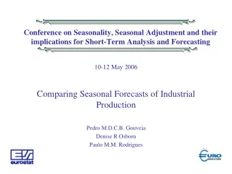
Conference on Seasonality, Seasonal Adjustment and their implications for Short-Term Analysis and Forecasting 10-12 May 2006 Comparison of Methods Accounting for Outliers during Seasonal Adjustment J. Aston Outliers SA Outliers Simulations
Conference on Seasonality, Seasonal Adjustment and their implications for Short-Term Analysis and Forecasting 10-12 May 2006 Comparison of Methods Accounting for Outliers during Seasonal Adjustment J. Aston
Outliers SA Outliers Simulations Real Data Summary References Comparison of Methods Accounting for Outliers during Seasonal Adjustment J. Aston Institute of Statistical Science Academia Sinica Eurostat Seasonal Adjustment Conference 2006 1
Outliers SA Outliers Simulations Real Data Summary References Outline Outliers Seasonal Adjustment Structural Component Models ARIMA models Outliers Gaussian Methods Non-Gaussian Methods Simulations Real Data UK Housing Transactions US Automobile Retail Series US Material Handling Equipment Manufacturing Series Summary 2
Outliers SA Outliers Simulations Real Data Summary References Data 30 25 20 15 10 5 0 1 2 3 4 5 6 7 8 3
Outliers SA Outliers Simulations Real Data Summary References Data Gauss Seasonal Adjustment 30 25 20 15 10 5 0 1 2 3 4 5 6 7 8 4
Outliers SA Outliers Simulations Real Data Summary References Model Based Seasonal Adjustment Use a component model to define a seasonal component and then remove this estimated component from the data. y sa = y t − S t t S t can be defined in many ways and is also dependent on all the other components in the model. The Unobserved Component models often define S t is terms of trigonometric functions, while ARIMA decomposition models give constrained ARIMA model representations. 5
Outliers SA Outliers Simulations Real Data Summary References Structural Component Models The Trig-1 seasonal model, with seasonal period s , is defined as [ s / 2 ] � S t = S j , t j = 1 S j , t = S j , t − 1 cos λ j + S ∗ j , t − 1 sin λ j + ω j , t S ∗ = − S j , t − 1 sin λ j + S ∗ j , t − 1 cos λ j + ω ∗ j , t j , t ω ) and λ j = 2 π j j , t ∼ N ( 0 , σ 2 and ω j , t , ω ∗ s . In addition, the local level model, T t = T t − 1 + η t where η t ∼ N ( 0 , σ 2 η ) , for the Trend specification, and a white noise Gaussian irregular component (with variance σ 2 ξ ). 6
Outliers SA Outliers Simulations Real Data Summary References ARIMA models Airline Model Basics ( 1 − B )( 1 − B s ) y t = ( 1 − θ B )( 1 − Θ B s ) ξ t Using the Hillmer-Tiao decomposition we can find (for suitable parameters) ( 1 − B ) 2 T t = θ T ( B ) ω t U ( B ) S t = θ S ( B ) η t I t = ε t where U ( B ) = ( 1 + B + . . . + B s − 1 ) and ω t , η t , ǫ t are white noise processes then y t = S t + T t + I t 7
Outliers SA Outliers Simulations Real Data Summary References Gaussian Outlier Adjustment - Simple Procedure 1. Set Outlier Threshold 2. Check Residuals - perform t-test 3. Include most significant term in model 4. Repeat 2. and 3. until no further significant terms 5. Check current outliers are still applicable 8
Outliers SA Outliers Simulations Real Data Summary References Gaussian Outlier Identification Simulation Variance Estimation for the differenced process 1.20 1.15 1.10 1.05 1.00 0.95 0.90 0.85 0 1 2 3 4 5 100 Simulated series (143 observations of monthly data) with 3 outliers. Histogram of estimated variance parameters (true value is 1 . 0) based on number of outliers detected by automatic Gaussian procedure (threshold value is 3 . 0) 9
Outliers SA Outliers Simulations Real Data Summary References Non Gaussian Components t ∼ t ( 0 , σ 2 I ∗ ξ , ν ) , t = 1 , . . . , n , where ν > 2 is the number of degrees of freedom and σ 2 ξ is the variance, which is constant for any ν . The decomposition model with a t-distributed irregular term can be expressed in its canonical form by t ∼ t ( 0 , σ 2 y t = S t + T t + I ∗ I ∗ ξ , ν ) , t = 1 , . . . , n . t , where t ( 0 , σ 2 ξ , ν ) refers to the t density. Structural Component Model: Estimate σ ξ , ν AMB Component Model: Estimate ν . Overall model gives σ ξ 10
Outliers SA Outliers Simulations Real Data Summary References Simulation Setup • 144/156 Series for both SC and AMB models • Three outliers at 5 times sd of Irr / No outliers added • Gaussian / Non-Gaussian Model Estimation • Mean Squared Seasonal Difference between 144/156 data lengths measured for 144 coincident points. 11
Outliers SA Outliers Simulations Real Data Summary References Comparison Histograms Seasonal Stability Seasonal Stability 15.0 45 12.5 40 35 10.0 30 25 7.5 20 5.0 15 10 2.5 5 -10 -5 0 5 10 15 20 25 30 -5.0 -2.5 0.0 2.5 5.0 7.5 10.0 12.5 15.0 17.5 Trig-1 Three Outliers Trig-1 No Outliers Seasonal Stability Seasonal Stability 15.0 25 12.5 20 10.0 15 7.5 10 5.0 5 2.5 -2.5 -2.0 -1.5 -1.0 -0.5 0.0 0.5 1.0 1.5 2.0 2.5 3.0 3.5 4.0 4.5 5.0 5.5 -0.25 0.00 0.25 0.50 0.75 1.00 1.25 1.50 1.75 2.00 AMB Three Outliers AMB No Outliers 12
Outliers SA Outliers Simulations Real Data Summary References England and Wales Housing Transactions Series 180 UK Housing Transactions Series 170 160 150 140 130 120 110 100 90 80 1995 2000 2005 13
Outliers SA Outliers Simulations Real Data Summary References Trig-1 Model Seasonal - Orig + 12months Seasonal - Orig Difference between Seasonals 0.05 0.2 0.00 0.0 -0.05 -0.10 -0.2 0 50 100 150 0 50 100 150 Seasonal - Orig + 12months Seasonal - Orig Difference between Seasonals 0.05 0.2 0.00 0.0 -0.05 -0.10 -0.2 0 50 100 150 0 50 100 150 14
Outliers SA Outliers Simulations Real Data Summary References AMB Model Seasonal - Orig + 12months Seasonal - Orig Difference between Seasonals 0.05 0.1 0.0 0.00 -0.1 -0.05 0 50 100 150 0 50 100 150 Seasonal - Orig + 12months Seasonal - Orig Difference between Seasonals 0.05 0.1 0.0 0.00 -0.1 -0.05 0 50 100 150 0 50 100 150 15
Outliers SA Outliers Simulations Real Data Summary References US Automobile Retail Series US Automobile Retail Series 80000 70000 60000 50000 40000 1995 2000 2005 16
Outliers SA Outliers Simulations Real Data Summary References Trig-1 Model 0.10 0.01 Seasonal - Orig + 12months Seasonal - Orig Difference between Seasonals 0.05 0.00 0.00 -0.05 -0.10 -0.01 0 50 100 150 0 50 100 150 0.10 0.01 Seasonal - Orig + 12months Seasonal - Orig Difference between Seasonals 0.05 0.00 0.00 -0.05 -0.10 -0.01 0 50 100 150 0 50 100 150 17
Outliers SA Outliers Simulations Real Data Summary References AMB Model 0.10 Seasonal - Orig + 12months Seasonal - Orig 0.003 Difference between Seasonals 0.002 0.05 0.001 0.00 0.000 -0.05 -0.001 -0.10 -0.002 0 50 100 150 0 50 100 150 0.003 Seasonal - Orig + 12months Seasonal - Orig Difference between Seasonals 0.10 0.002 0.05 0.001 0.00 0.000 -0.05 -0.001 -0.10 -0.002 0 50 100 150 0 50 100 150 18
Outliers SA Outliers Simulations Real Data Summary References US Material Handling Equipment Manufacturing Series 2500 US Material Handling Equipment Manufacturing Series 2250 2000 1750 1500 1250 1000 1995 2000 2005 19
Outliers SA Outliers Simulations Real Data Summary References Trig-1 Model 0.050 Seasonal - Orig + 12months Seasonal - Orig Difference between Seasonals 0.2 0.025 0.1 0.000 0.0 -0.1 -0.025 0 50 100 150 0 50 100 150 Seasonal - Orig + 12months Seasonal - Orig 0.050 Difference between Seasonals 0.2 0.025 0.1 0.000 0.0 -0.1 -0.025 0 50 100 150 0 50 100 150 20
Outliers SA Outliers Simulations Real Data Summary References AMB Model 0.002 Seasonal - Orig + 12months Seasonal - Orig Difference between Seasonals 0.2 0.001 0.1 0.000 0.0 -0.001 -0.002 -0.1 0 50 100 150 0 50 100 150 0.002 Seasonal - Orig + 12months Seasonal - Orig Difference between Seasonals 0.2 0.001 0.1 0.000 0.0 -0.001 -0.002 -0.1 0 50 100 150 0 50 100 150 21
Outliers SA Outliers Simulations Real Data Summary References Summary • Critical values can lead to unstable seasonals • Non-Gaussian models give reasonable seasonals when no outliers present • Non-Gaussian models reduce instability when outliers present • Caveats: • More Parameters needed • Computationally more intensive 22
Outliers SA Outliers Simulations Real Data Summary References References I Aston, J. A. D. and S. J. Koopman (2006). A non-gaussian generalisation of the airline model for robust seasonal adjustment. Journal of Forecasting , in press. Bruce, A. G. and S. R. Jurke (1996). Non-Gaussian seasonal adjustment: X-12-ARIMA versus robust structural models. Journal of Forecasting 15 , 305–328. Gómez, V. and A. Maravall (2001a). Automatic modeling methods for univariate series. In D. Peña, G. C. Tiao, and R. S. Tsay (Eds.), A Course in Time Series . New York, NY: J. Wiley and Sons. Chapter 7. 23
Recommend
More recommend
Explore More Topics
Stay informed with curated content and fresh updates.
