Computational Learning Theory For which tasks is successful learning - PDF document

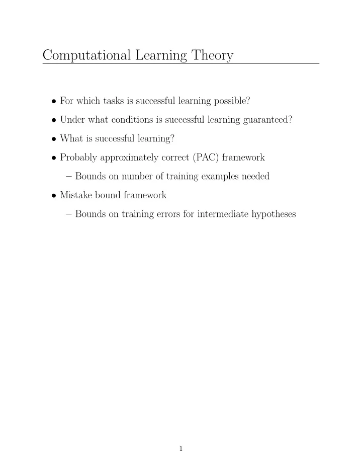
Computational Learning Theory • For which tasks is successful learning possible? • Under what conditions is successful learning guaranteed? • What is successful learning? • Probably approximately correct (PAC) framework – Bounds on number of training examples needed • Mistake bound framework – Bounds on training errors for intermediate hypotheses 1

Problem • Given – Size or complexity of hypothesis space considered by learner – Accuracy to which target concept must be approximated – Probability that learner will output successful hypothesis – Manner in which training examples presented to learner • Find – Sample complexity ∗ Number of training examples needed for learner to con- verge (with high probability) to successful hypothesis – Computational complexity ∗ Amount of computational effort needed for learner to con- verge (with high probability) to successful hypothesis – Mistake bound ∗ Number of training examples misclassified by learner be- fore converging to successful hypothesis 2

Problem Details • Successful hypothesis – Equals target concept – Usually agrees with target concept • How training examples obtained – Helpful teacher (near misses) – Learner-generated queries – Random sample 3

Probably Learning an Approximately Correct Hypothesis • Probably approximately correct (PAC) learning model • E.g., boolean-valued concepts from noise-free training data • Problem setting – X = set of all possible instances – C = set of possible target concepts ∗ Each c ∈ C corresponds to boolean-valued function c : X → { 0 , 1 } ∗ c ( x ) = 1 → positive example ∗ c ( x ) = 0 → negative example – Instances randomly sampled from X according to prob. dis- trib. D ∗ D is stationary (does not change over time) – Training examples consist of � x, c ( x ) � ∗ x randomly drawn from X according to D – Learner L considers possible hypotheses from H – Learner’s output h evaluated on randomly drawn test set from X by D – Looking for successful combinations of L , H and C – Worst case analysis for all possible C and D 4

Error of Hypothesis Instance space X - - c h + + - Where c and h disagree • True error ( error D ( h )) – Of hypothesis h with respect to target concept c and distri- bution D is the probability that h will misclassify an instance drawn at random according to D – error D ( h ) = Pr x ∈D ( c ( x ) � = h ( x )) • D can be any distribution, not necessarily uniform • L can only see training examples • Training error = fraction of training examples misclassified by h • Analysis centers around how well training error estimates true error 5

PAC Learnability • What classes of target concepts can be reliably learned with a reasonable amount of time and training examples? • Learnability constraints – error D ( h ) = 0 ∗ Impossible unless we see entire X ∗ Small chance training sample is misleading – error D ( h ) ≤ ǫ ∗ Probability of failure ≤ δ ∗ I.e., probably learn approximately correct hypothesis (PAC) 6

Definition • Given concept class C over instances X of length n and learner L using hypothesis space H , C is PAC-Learnable by L using H if ∀ c ∈ C , ∀ distributions D over X , ∀ ǫ such that 0 < ǫ < 1 / 2, and ∀ δ such that 0 < δ < 1 / 2, learner L will with probability (1 − δ ) output a hypothesis h ∈ H such that error D ( h ) ≤ ǫ , in time polynomial in 1 /ǫ , 1 /δ , n and size ( c ). • n = size of an instance (e.g., number of boolean attributes) • size ( c ) = length of some encoding of elements in C • Definition limits number of training examples to be polynomial too 7

Sample Complexity for Finite Hypothesis Spaces • Sample complexity – Number of training examples needed for learner to produce PAC hypothesis • Sample complexity for consistent learner – Consistent learner ∗ Outputs hypothesis with no errors on training data (when possible) • Bound on sample complexity of ANY consistent learner – Recall version space V S H,D ∗ V S H,D = { h ∈ H |∀� x, c ( x ) � ∈ D ( h ( x ) = c ( x )) } – Every consistent learner outputs h ∈ V S H,D for any X , H and D – Bound number of examples to find consistent V S H,D 8

ǫ -Exhausted Version Space Hypothesis space H error =.3 error =.1 r =.4 r =.2 error =.2 r =0 VSH,D error =.2 error =.3 r =.3 error =.1 r =.1 r =0 ( r = training error, error = true error) • Given hypothesis space H , target concept c , instance distribu- tion D , and set of training examples D of c , version space V S H,D is ǫ -exhausted with respect to c and D , if every hypothesis h ∈ V S H,D has error less that ǫ with respect to c and D . ∀ h ∈ V S H,D ( error D ( h ) < ǫ ) • Can bound the probability that V S H,D is ǫ -exhausted after some number of training examples 9

Thm. 7.1 ǫ -Exhausting the Version Space • If hypothesis space H is finite, and D is a sequence of m ≥ 1 independent randomly drawn examples of some target concept c , then for any 0 ≤ ǫ ≤ 1, the probability that the version space V S H,D is not ǫ -exhausted (with respect to c ) is ≤ | H | e ( − ǫm ) • Proof: – Let h 1 , ..., h k be hypotheses in H with error > ǫ w.r.t. c – To not ǫ -exhaust V S H,D , one of h i would be in V S H,D ∗ I.e., h i consistent with all m training examples ∗ Probability = (1 − ǫ ) m – Probability that one of h i ∈ V S H,D is k (1 − ǫ ) m – Since k ≤ | H | , k (1 − ǫ ) m ≤ | H | (1 − ǫ ) m – Since (1 − ǫ ) ≤ e − ǫ , | H | (1 − ǫ ) m ≤ | H | e ( − ǫm ) ✷ • Result: – Want | H | e ( − ǫm ) ≤ δ ∗ Sample complexity m ≥ (1 /ǫ )(ln | H | + ln(1 /δ )) – Given this many training examples, any consistent learner will output a hypothesis that is probably approximately cor- rect ∗ Typically overestimates sample complexity due to | H | 10

Agnostic Learner • Finds hypothesis with minimum training error when c �∈ H • Pr [ error D ( h ) > error D ( h ) + ǫ ] ≤ e ( − 2 mǫ 2 ) • Pr [( ∃ h ∈ H )( error D ( h ) > error D ( h ) + ǫ )] ≤ | H | e ( − 2 mǫ 2 ) • Letting this probability be δ – m ≥ (1 / 2 ǫ 2 )(ln | H | + ln(1 /δ )) – m grows with square of 1 /ǫ instead of linearly as before 11

Example C = conjunctions of boolean literals ( a or ¬ a ) • Is C PAC learnable? – Show poly number of training examples for any c ∈ C – Design consistent learner using poly time per training exam- ple • | H | = 3 n for n boolean attributes – m ≥ (1 /ǫ )( n ln 3 + ln(1 /δ )) – E.g., n = 10, δ = 0 . 05, ǫ = 0 . 1, m ≥ 140 – E.g., n = 10, δ = 0 . 01, ǫ = 0 . 01, m ≥ 1560 • Algorithm Find-S is a consistent, poly time learner • Thus C is PAC-learnable by Find-S with H = C 12

How About EnjoySport ? m ≥ 1 ǫ (ln | H | + ln(1 /δ )) If H is as given in EnjoySport then | H | = 973, and m ≥ 1 ǫ (ln 973 + ln(1 /δ )) If want to assure that with probability 95%, V S contains only hypotheses with error D ( h ) ≤ . 1, then it is sufficient to have m examples, where m ≥ 1 . 1(ln 973 + ln(1 /. 05)) m ≥ 10(ln 973 + ln 20) m ≥ 10(6 . 88 + 3 . 00) m ≥ 98 . 8 13

PAC-Learnability of Other Concept Classes • Unbiased concept class | C | = 2 | X | – E.g., for n boolean attributes, | X | = 2 n – If H = C , then | H | = 2 (2 n ) – m ≥ (1 /ǫ )(2 n ln 2 + ln(1 /δ )) ∗ Exponential in n ⇒ not PAC learnable ∗ Can be proven that m = Θ(2 n ) • k -term DNF – Concept form T 1 ∨ T 2 ∨ ... ∨ T k ∗ Each T i conjunction of literals from n boolean attributes – | H | = (3 n ) k = 3 nk ∗ Overestimate: includes cases where T i = T j and T i > g T j – m ≥ (1 /ǫ )( nk ln 3 + ln(1 /δ )) – However, learning k -term DNF is NP-hard – Thus, not PAC-learnable when H = k -term DNF, but ... • k -CNF – Concept form T 1 ∧ ... ∧ T j for arbitrarily large j ∗ Each T i is a disjunction of k literals – k -CNF has poly time learner and sample complexity – Thus, H = k -CNF is PAC-learnable – Since any k -term DNF can be written as a k -CNF, k -term DNF is PAC-learnable by H = k -CNF 14

Sample Complexity for Infinite Hypothesis Spaces • Weakness in above result – Weak bound – Inapplicable for infinite H • Consider second measure of complexity of H (other than | H | ) – Vapnik-Chervonenkis (VC) dimension of H , V C ( H ) – Tighter than above bound – Finite for some infinite H ’s 15

Shattering a Set of Instances • Number of distinct instances of X that can be completely dis- criminated using H • Given sample S from X – There are 2 | S | possible dichotomies of S – I.e., 2 | S | different ways of assigning (+,-) classes to members of S • H shatters S if every possible dichotomy of S can be expressed by some hypothesis from H • Definition – A set of instances S is shattered by hypothesis space H iff for every dichotomy of S there exists some hypothesis in H consistent with this dichotomy Instance space X 16

VC Dimension • Ability to shatter related to inductive bias • Unbiased hypothesis space shatters X • What if H can shatter only some large subset of X ? – The larger this subset, the more expressive H is • VC dimension measures this expressiveness • Definition – V C ( H ) of hypothesis space H defined over instance space X is the size of the largest finite subset of X shattered by H . If arbitrarily large subsets of X can be shattered by H , then V C ( H ) = ∞ • For any finite H , V C ( H ) ≤ lg | H | – 2 d ≤ | H | , where d = V C ( H ) 17