Compression Programs File Compression: Gzip, Bzip Archivers :Arc, - PDF document

Compression Programs • File Compression: Gzip, Bzip • Archivers :Arc, Pkzip, Winrar, … • File Systems: NTFS Analysis of Algorithms Piyush Kumar (Lecture e 5: Compression) on) Welcome to 4531 Source: Guy E. Blelloch, Emad, Tseng … Multimedia Compression Outline • HDTV (Mpeg 4) Introduction : Lossy vs. Lossless • Sound (Mp3) Information Theory : Entropy, etc. • Images (Jpeg) Probability Coding : Huffman + Arithmetic Coding Lossless vs. 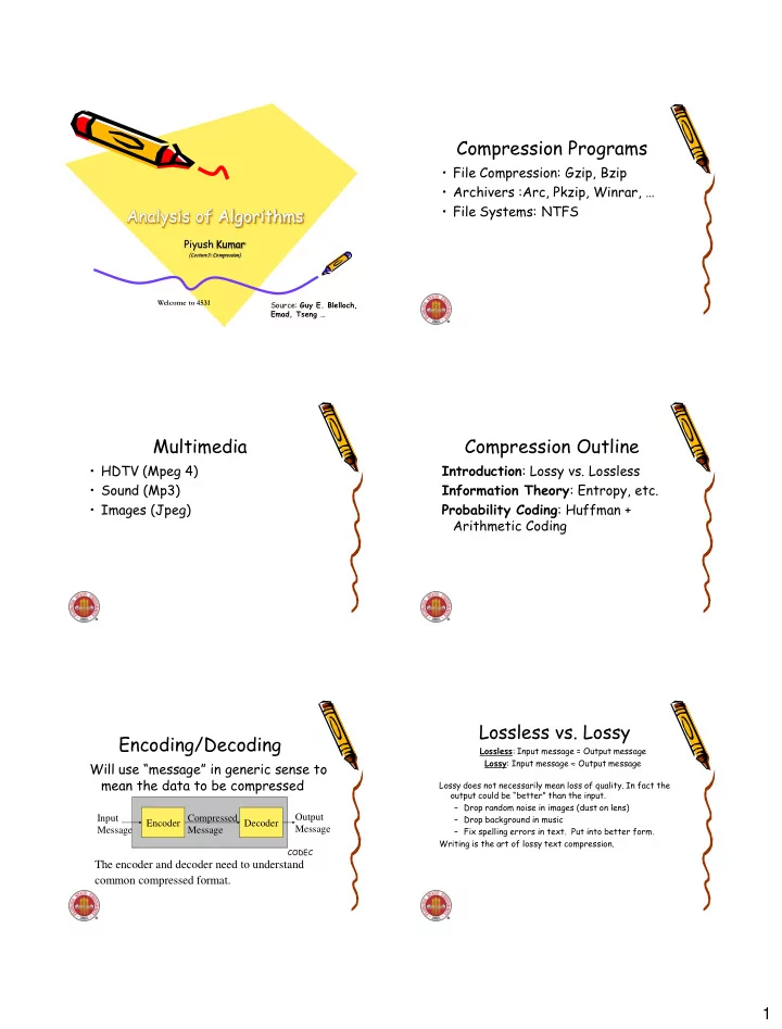Lossy Encoding/Decoding Lossless : Input message = Output message Lossy : Input message  Output message Will use “message” in generic sense to mean the data to be compressed Lossy does not necessarily mean loss of quality. In fact the output could be “better” than the input. – Drop random noise in images (dust on lens) Output Input Compressed – Drop background in music Encoder Decoder Message Message Message – Fix spelling errors in text. Put into better form. Writing is the art of lossy text compression. CODEC The encoder and decoder need to understand common compressed format. 1

Lossless Compression Techniques How much can we • LZW (Lempel-Ziv-Welch) compression compress? – Build dictionary For lossless compression, assuming all – Replace patterns with index of dict. input messages are valid, if even one • Burrows-Wheeler transform string is compressed, some other – Block sort data to improve compression must expand. • Run length encoding – Find & compress repetitive sequences • Huffman code – Use variable length codes based on frequency Model vs. Coder Quality of Compression To compress we need a bias on the probability of Runtime vs. Compression vs. Generality messages. The model determines this bias Several standard corpuses to compare algorithms Calgary Corpus Encoder • 2 books, 5 papers, 1 bibliography, 1 collection of news articles, 3 programs, Messages Probs. Bits Model Coder 1 terminal session, 2 object files, 1 geophysical data, 1 bitmap bw image The Archive Comparison Test maintains a comparison of just about all algorithms publicly Example models: available – Simple: Character counts, repeated strings – Complex: Models of a human face Comparison of Information Theory Algorithms An interface between modeling and coding • Entropy Program Algorithm Time BPC Score BOA PPM Var. 94+97 1.91 407 – A measure of information content PPMD PPM 11+20 2.07 265 • Entropy of the English Language IMP BW 10+3 2.14 254 – How much information does each character in “typical” English text BZIP BW 20+6 2.19 273 contain? GZIP LZ77 Var. 19+5 2.59 318 LZ77 LZ77 ? 3.94 ? 2

Entropy (Shannon 1948) Entropy Example For a set of messages S with probability p(s),  s  S , the self information of s is: p S ( ) {. 25 25 25 125 125 ,. ,. ,. ,. }      1 ( ) 3 25 . log 4 2 125 . log 8 2 25 . H S    i s ( ) log log ( ) p s p s ( )  ( ) {. ,. 5 125 125 125 125 ,. ,. ,. } p S Measured in bits if the log is base 2.     H S ( ) . log 5 2 4 125 . log 8 2 The lower the probability, the higher the information  ( ) {. 75 0625 0625 0625 0625 ,. ,. ,. ,. } p S Entropy is the weighted average of self     ( ) . 75 log( 4 3 ) 4 0625 . log 16 13 . H S information. 1   ( ) ( )log H S p s ( ) p s  s S Shannon’s experiment Entropy of the English Language How can we measure the information per Asked humans to predict the next character character? given the whole previous text. He used these as conditional probabilities to ASCII code = 7 estimate the entropy of the English Entropy = 4.5 (based on character Language. probabilities) The number of guesses required for right Huffman codes (average) = 4.7 answer: # of guesses 1 2 3 3 5 > 5 Unix Compress = 3.5 Probability .79 .08 .03 .02 .02 .05 Gzip = 2.5 BOA = 1.9 (current close to best text From the experiment he predicted compressor) H(English) = .6-1.3 Must be less than 1.9. Data compression model Coding How do we use the probabilities to Input data code messages? • Prefix codes and relationship to Reduce Data Redundancy Entropy Reduction of Entropy • Huffman codes • Arithmetic codes Entropy Encoding • Implicit probability codes… Compressed Data 3

Assumptions Uniquely Decodable Codes A variable length code assigns a bit string Communication (or file) broken up into pieces called (codeword) of variable length to every messages. message value Adjacent messages might be of a different types e.g. a = 1, b = 01, c = 101, d = 011 and come from a different probability What if you get the sequence of bits distributions 1011 ? We will consider two types of coding: • Discrete : each message is a fixed set of bits Is it aba, ca, or, ad ? – Huffman coding, Shannon-Fano coding A uniquely decodable code is a variable length • Blended : bits can be “shared” among messages code in which bit strings can always be – Arithmetic coding uniquely decomposed into its codewords. Prefix Codes Some Prefix Codes for Integers A prefix code is a variable length code in which no codeword is a prefix of n Binary Unary Split another word 1 ..001 0 1| e.g a = 0, b = 110, c = 111, d = 10 2 ..010 10 10|0 Can be viewed as a binary tree with 3 ..011 110 10|1 message values at the leaves and 0 or 1110 110|00 4 ..100 1s on the edges. 5 ..101 11110 110|01 0 1 6 ..110 111110 110|10 0 1 a Many other fixed prefix codes: 0 1 d Golomb, phased-binary, subexponential, ... b c Average Bit Length Relationship to Entropy For a code C with associated Theorem (lower bound): For any probabilities p(c) the average length probability distribution p(S) with is defined as associated uniquely decodable code C,   ( ) ( ) ( ) ABL C p c l c  ( ) ( ) H S ABL C  c C We say that a prefix code C is optimal Theorem (upper bound): For any if for all prefix codes C’, probability distribution p(S) with associated optimal prefix code C, ABL(C)  ABL(C’)   ABL ( C ) H ( S ) 1 4

Kraft McMillan Inequality Proof of the Upper Bound (Part 1)   Assign to each message a length    ( ) log 1 ( ) l s p s Theorem (Kraft-McMillan): For any uniquely We then have     decodable code C,      log 1 / ( )  ( ) p s 2 l s 2   ( ) 2 l c 1   s S s S     c C   log 1 / ( ) p s 2 Also, for any set of lengths L such that   s S   l  2 1  p s ( )  l L there is a prefix code C such that  s S  1   1 ( ) ( ,...,| |) l c l i L So by the Kraft-McMillan ineq. there is a i i prefix code with lengths l(s) . Another property of optimal codes Proof of the Upper Theorem: If C is an optimal prefix code for Bound (Part 2) the probabilities {p 1 , …, p n } then p i > p j implies l(c i )  l(c j ) Now we can calculate the average length given l(s)   Proof: (by contradiction) ( ) ( ) ( ) ABL S p s l s Assume l(c i ) > l(c j ). Consider switching  s S        ( ) log 1 / ( ) p s p s codes c i and c j . If l a is the average length  s S of the original code, the length of the new     ( ) ( 1 log( 1 / ( ))) p s p s code is  s S    1 ( ) log( 1 / ( )) p s p s      ' ( ( ) ( )) ( ( ) ( )) l l p l c l c p l c l c a a j i j i j i  s S       ( )( ( ) ( )) l p p l c l c 1 ( ) H S a j i i j  l This is a contradiction since l a was And we are done. a supposed to be optimal Corollary • The p i is smallest over the code, then l(c i ) is the largest. Huffman Coding Binary trees for compression 5